Building an LLM Load Test That Reflects Real Traffic

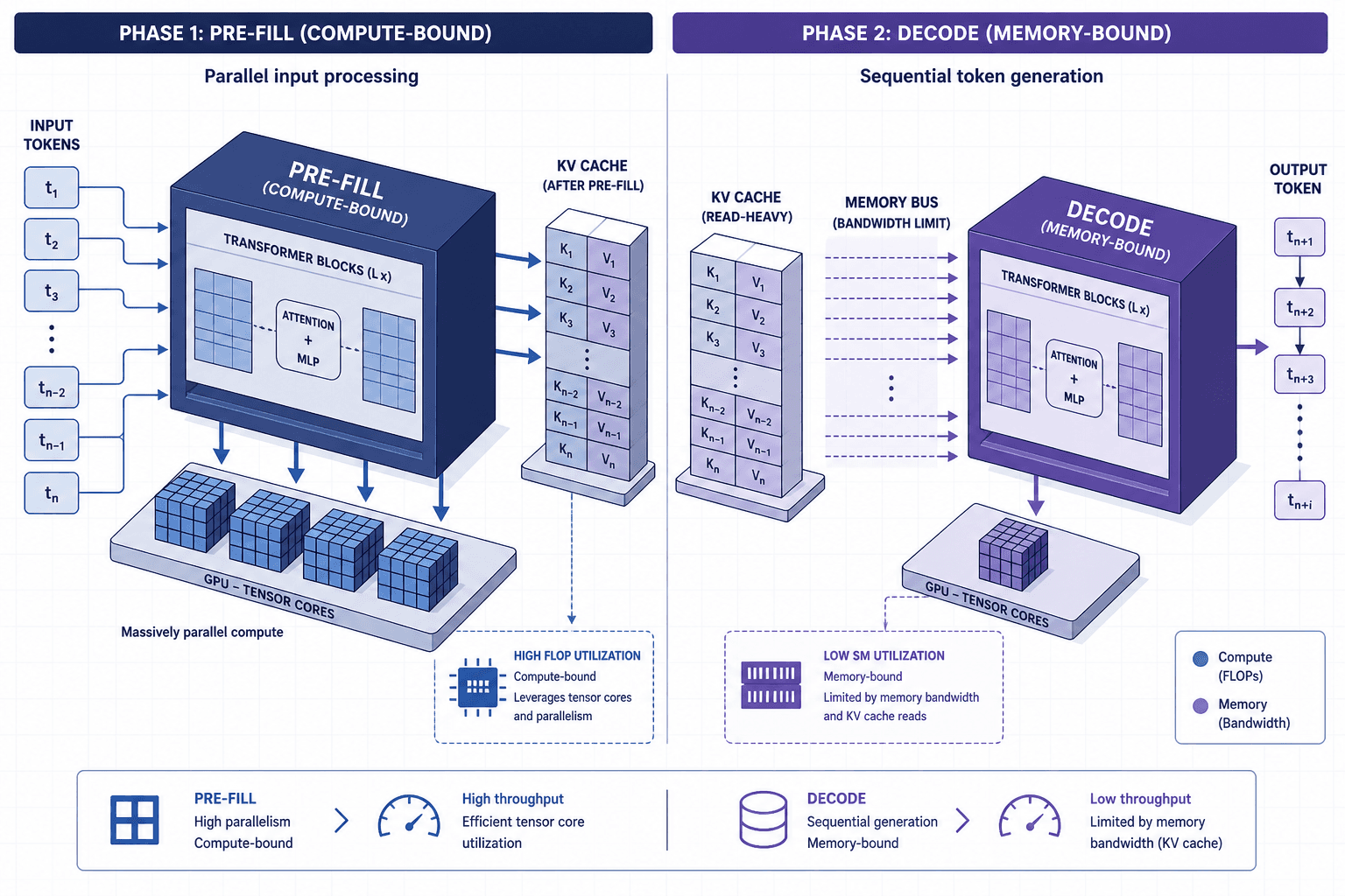
Standard load testing tools like k6, Locust, or JMeter are engineered for stateless HTTP endpoints, assuming a request arrives, is processed, and returns within a predictable window. Large Language Models (LLMs) fundamentally break this assumption. An LLM request is not a single atomic operation but a two-phase process with distinct performance characteristics: the pre-fill phase and the decode phase. Achieving realistic traffic simulation requires understanding that these phases have different bottlenecks—compute-bound versus memory-bound—which standard RPS metrics fail to capture individually. Testing an LLM using standard Request Per Second (RPS) targets without accounting for this split yields misleading results. You might achieve 100 RPS in a test environment, yet that same load could cause a cascading failure in production because the test failed to simulate the memory-bound bottleneck inherent in token generation. To build a robust evaluation framework, you must model the queue dynamics of these two phases separately, applying capacity planning principles specific to generative AI workloads.

The Two-Phase Bottleneck Mechanism

When an LLM receives a prompt, it executes two distinct computational steps. Understanding the mechanism of each is critical for defining accurate test parameters.

1. The Pre-fill Phase (Compute-Bound)

The system takes the entire input prompt (e.g., 1,000 tokens) and processes it in parallel across GPU tensor cores to generate the key-value (KV) cache. This phase is highly parallelizable. If you double the batch size, the time to complete the pre-fill increases only marginally because the operation remains compute-bound and highly parallelizable, with spare GPU compute capacity absorbing the additional load rather than being constrained by memory bandwidth.

2. The Decode Phase (Memory-Bound)

Once the KV cache is built, the model generates output tokens one by one. For each new token, the model must attend to all previous tokens (including the prompt and previously generated tokens). This is sequential. You cannot generate token $N+1$ until token $N$ is computed. This phase is strictly memory-bandwidth bound. The GPU sits idle waiting for data to move from VRAM to the ALU.

The Failure Mode: Standard load tests often hit the pre-fill limit first. They send 1,000 requests simultaneously. The GPU handles the parallel pre-fill fine. However, if each request generates 500 tokens, the GPU must now manage 500,000 sequential decode steps. If the test tool releases the connection after the pre-fill or assumes a fixed latency, it misses the fact that the GPU is now completely saturated by memory bandwidth, not compute. The queue depth explodes, and latency spikes dramatically.

Modeling Arrival Rates with Little’s Law

To reflect real traffic, you must calculate the concurrency your system can handle, not just the RPS. Real traffic is rarely uniform; it is bursty. However, the sustaining load is determined by the decode phase.

We use Little’s Law to determine the maximum sustainable concurrency ($L$) before the system saturates:

$$L = \lambda \times W$$

Where:

• $\lambda$ (Lambda) is the arrival rate (requests per second).
• $W$ (Wait time) is the average time a request spends in the system (TTFT + generation time).

In an LLM context, $W$ is dominated by the decode phase. Let's work through a concrete scenario.

Scenario:

• Model: Llama-3-70B on A100 80GB.
• Average Prompt Length: 500 tokens.
• Average Response Length: 200 tokens.
• Measured Decode Speed: 50 tokens/second (t/s).

Step 1: Calculate Time per Request ($W$)

• TTFT (Pre-fill): ~0.5 seconds (negligible compared to decode).
• Generation Time: 200 tokens / 50 t/s = 4.0 seconds.
• Total $W$ ≈ 4.5 seconds.

Step 2: Determine Saturation Point ($L$) Assume your GPU cluster can sustain a maximum decode throughput of 2,000 tokens/second before hitting memory bandwidth walls.

• Max $\lambda$ (Throughput) = 2,000 t/s.
• Since each request generates 200 tokens, the max sustainable RPS is $2,000 / 200 = 10$ RPS.
• Using Little’s Law: $L = 10 \text \times 4.5 \text = 45$ concurrent requests.

Note: Little’s Law provides an upper bound or approximation. Actual concurrency limits depend on the specific batching strategy and scheduler (e.g., vLLM's continuous batching) which may allow higher concurrency than the simple formula suggests due to variable service times.

If your load test sends 100 concurrent requests, you are exceeding the saturation point. The queue will grow indefinitely until the server times out. A standard RPS test that doesn't cap concurrency at 45 will fail to show you the graceful degradation curve; it will just show a hard crash.

Simulating Bursty Traffic

Real user traffic is not a steady stream. It follows a Poisson distribution with bursts. To simulate this, you cannot simply send requests at a constant interval. You must use a step-load or spike pattern that respects the concurrency limit calculated above.

Here is how to structure the load profile in a tool like k6 or Locust:

// Pseudo-code for realistic LLM load profile
function scenario() {
  // 1. Warmup: Ramp up to 80% of calculated saturation (45 * 0.8 = 36 concurrent)
  // This ensures we test the stable region before the cliff.
  const maxConcurrent = 36;
  
  // 2. Arrival Pattern: Poisson-distributed arrivals
  // Instead of fixed intervals, use random delays between requests
  // that sum up to the target RPS, but allow for bursts.
  sleep(random(0.1, 0.5)); // Variable delay
  
  // 3. Request Execution
  http.post("/v1/chat/completions", {
    body: JSON.stringify({
      model: "llama-3",
      messages: [{ role: "user", content: "..." }],
      max_tokens: 200,
      stream: false // Test sync first to measure total latency
    })
  });
  
  // 4. Critical Check: Monitor Queue Depth
  // If the response time exceeds W * 2, the system is queuing.
  if (httpResponse.timings.duration > 9000) { // 9s is 2x expected 4.5s
    log("System is queuing: Latency spike detected");
  }
}

Saturation Metrics: Beyond Error Rates

In traditional web apps, a 5xx error indicates failure. In LLM systems, the system may never return a 5xx error during saturation; it will simply return responses with increasing latency until the client times out. You need specific saturation metrics to detect soft saturation.

1. Time-to-First-Token (TTFT) Stability

During the pre-fill phase, TTFT should remain stable. It is crucial to distinguish between computation time and queuing delay. TTFT reflects the health of the pre-fill queue, comprising both the actual pre-fill computation time and any delay caused by waiting in line for GPU resources. If TTFT starts increasing linearly with load, it indicates that the pre-fill queue is full. This is a compute-bound issue. You can often mitigate this by adding more GPUs for pre-fill (if using a distributed architecture like vLLM).

2. Tokens-Per-Second (TPS) Decay

This is the most critical metric. As you increase load, the TPS per request should remain constant until the GPU hits memory bandwidth limits. Once saturated, TPS will drop. If TPS drops, it means the system is spending more time managing memory access than generating tokens. This is a hardware limit that cannot be solved by adding more application servers; you need more VRAM or faster memory.

3. Queue Depth

You can estimate queue depth by comparing the arrival rate to the processing rate. If your arrival rate is 10 RPS and your processing rate is 10 RPS, the queue should be stable. If the arrival rate is 11 RPS, the queue grows by 1 request per second. In a production monitoring system (like Prometheus), you can track the number of active inference sessions. A growing count of active sessions without a corresponding drop in TPS indicates imminent saturation.

Conclusion

Building an LLM load test that reflects real traffic requires abandoning the "RPS-first" mindset. You must treat the LLM as a two-phase machine with a memory-bound bottleneck. By calculating concurrency using Little’s Law based on the decode phase duration, and by monitoring TPS decay and queue depth, you can identify the true saturation point of your system. This approach prevents the common pitfall of over-provisioning compute for pre-fill while under-provisioning for the memory-intensive decode phase, ensuring your infrastructure scales correctly under real-world load. Crucially, this method addresses the two separate queues—pre-fill and decode—ensuring that bottlenecks in either stage are visible and measurable, rather than hidden by aggregate latency metrics.

Common Pitfalls

1. Ignoring Decode Saturation: Focusing solely on TTFT or initial request handling while neglecting the sustained memory bandwidth constraints of the decode phase. This leads to systems that handle initial load well but fail catastrophically under sustained generation.
2. Misinterpreting TTFT: Assuming an increase in TTFT is always a compute bottleneck. As clarified, TTFT increases can also signal queuing delays in the pre-fill stage, which requires different scaling strategies (e.g., more pre-fill nodes) than compute upgrades.
3. Assuming Linear Scaling: Believing that adding more GPUs will linearly improve throughput. Due to memory bandwidth limits and KV cache overheads, scaling is often non-linear, especially for long context windows where memory access becomes the dominant constraint.

Practical Takeaways

• Model Two Phases Separately: Always analyze pre-fill (compute) and decode (memory) performance independently.
• Use Little’s Law for Concurrency: Calculate max concurrency based on decode time, not just RPS, to avoid queue explosion.
• Monitor TPS Decay: Use Tokens-Per-Second as the primary indicator of memory-bound saturation, not just error rates.

FAQ

Q: Can I use standard RPS tools for LLM load testing? A: You can use them, but you must configure them to respect concurrency limits derived from decode times. Simply setting a high RPS will likely overwhelm the system by ignoring the two-phase nature of inference.

Q: How do I distinguish between pre-fill and decode bottlenecks? A: Monitor TTFT and TPS. If TTFT increases but TPS remains stable, the bottleneck is likely in the pre-fill queue (compute-bound). If TTFT is stable but TPS drops, the bottleneck is in the decode phase (memory-bound).

Q: Does batching help with decode saturation? A: Yes, continuous batching (like in vLLM) can improve utilization by filling gaps between token generations, but it cannot overcome the physical limits of memory bandwidth. Eventually, adding more requests will still degrade TPS if the GPU is memory-saturated.