Continuous Batching, Illustrated

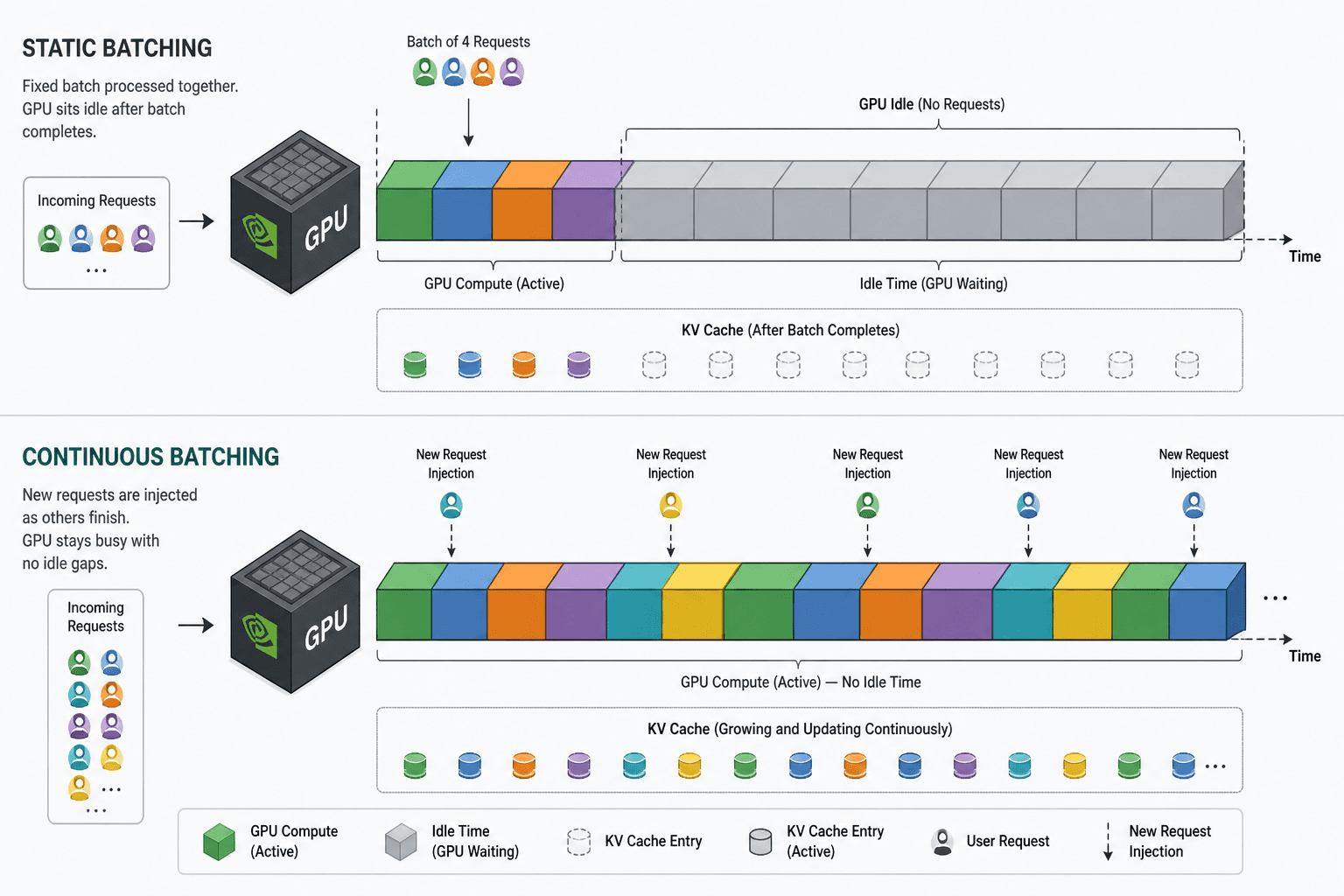
In Large Language Model (LLM) inference, throughput is not just about how fast the GPU computes; it is about how efficiently the GPU is utilized between computations. The primary bottleneck in naive inference systems is not compute, but latency variation. Different user requests generate different numbers of output tokens. In a traditional static batching setup, the system must wait for the slowest request in the batch to finish before starting the next batch. This creates significant idle time where the GPU sits empty, wasting money and reducing capacity.

Continuous batching, also known as iteration-level scheduling, solves this by treating the batch as a dynamic pool of active sequences rather than a fixed grid of padded inputs. This approach, popularized by systems like Orca and implemented in modern frameworks like vLLM and SGLang, allows the scheduler to inject new requests into the batch the moment any existing request completes, maximizing GPU utilization.

The Problem with Static Batching

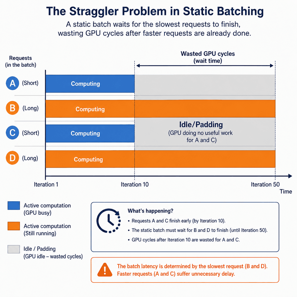
To understand continuous batching, we must first visualize the failure mode of static batching. Imagine a batch size of 4. Four users send requests: A, B, C, and D.

• Request A generates 10 tokens.
• Request B generates 50 tokens.
• Request C generates 10 tokens.
• Request D generates 50 tokens.

In static batching, the system processes these in fixed iterations. In iteration 1, the GPU computes the first token for all four requests. In iteration 2, it computes the second token for all four. This continues until iteration 10. At this point, requests A and C have finished generating their output. However, the system cannot discard them or start new work yet. It must continue processing iterations 11 through 50, where A and C are effectively "padding" data—zeros or no-ops—while the GPU computes for B and D.

This is inefficient. The GPU spends 80% of its time (iterations 11–50) computing nothing useful for A and C. If there were a queue of new requests waiting, they would sit idle. This is the "straggler problem": the batch duration is determined by the maximum length of any request in the batch, not the average.

The Mechanism: Iteration-Level Scheduling

Dynamic batching, often referred to as iteration-level scheduling, changes the unit of scheduling from the batch to the iteration (or step). The scheduler maintains a list of active sequences, each with its own independent state. Crucially, it decouples the generation of new tokens from the synchronization of the entire batch.

The core mechanism relies on the Key-Value (KV) Cache. When an LLM processes a sequence, it computes attention over previous tokens. The results (Keys and Values) are stored in memory so they don't need to be recomputed for subsequent tokens. In static batching, the KV cache is often allocated as a contiguous block padded to the maximum sequence length. In continuous batching, the KV cache is managed per-sequence, allowing variable lengths. This concept is foundational to systems like PagedAttention, which optimizes memory management by treating the KV cache as a set of non-contiguous blocks.

Here is how the scheduler operates in a concrete scenario with actors Alice, Bob, and Charlie.

Step 1: Initial State

The scheduler has a batch capacity of 4. Currently, it holds:

• Alice: Generated 5 tokens. Needs 10 more.
• Bob: Generated 5 tokens. Needs 10 more.
• Charlie: Generated 5 tokens. Needs 10 more.
• Slot 4: Empty.

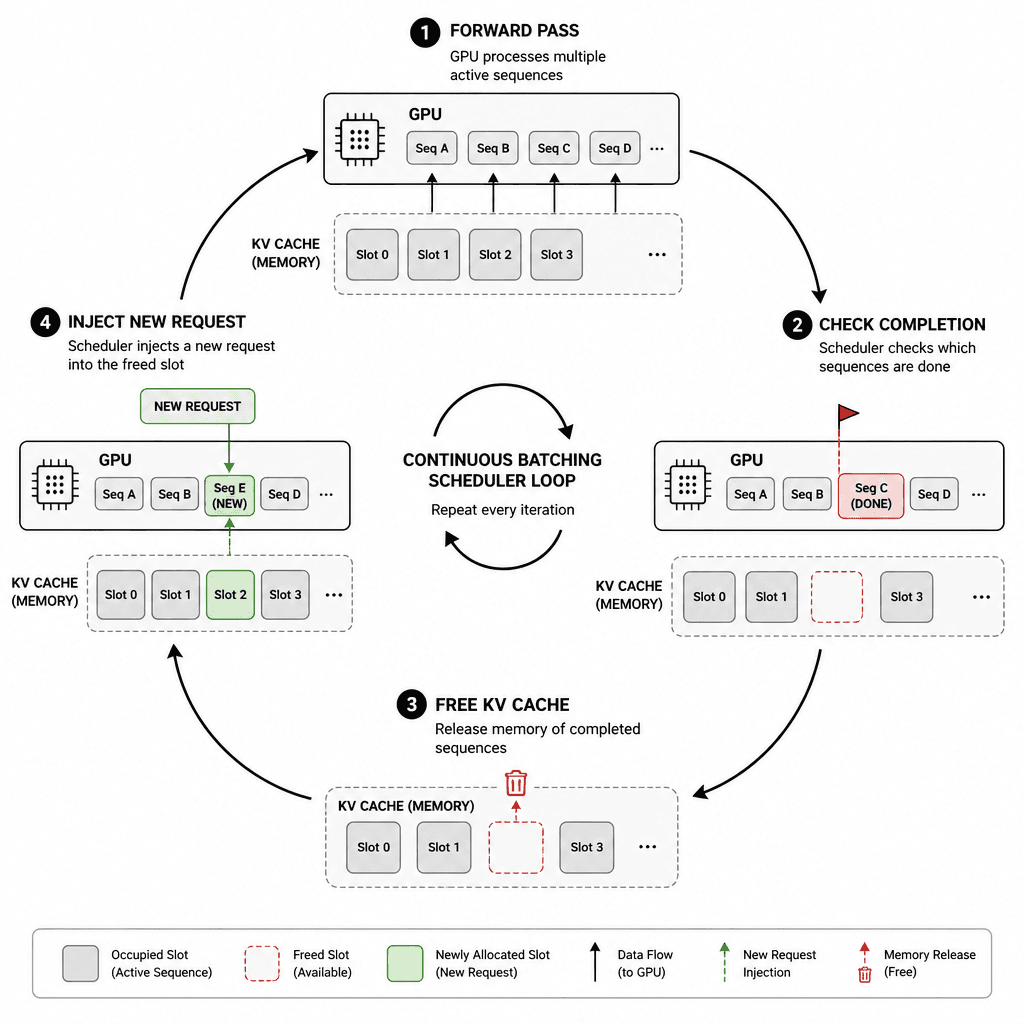
Step 2: The Forward Pass

The GPU runs a forward pass for the current tokens of Alice, Bob, and Charlie. This produces the next token for each. The system updates their internal states.

Step 3: Completion Check

After the forward pass, the scheduler checks which sequences have reached their maximum generation limit or stopped (e.g., via EOS token). Suppose Alice finishes her generation after this step. She is now "done."

Step 4: Resource Reclamation

Because Alice is done, the system frees the KV cache slots that belonged to her. These slots are now available for new incoming requests. The scheduler does not wait for Bob or Charlie to finish. It immediately looks at the request queue.

Step 5: Injection

A new request, Dave, arrives. The scheduler sees that one slot is free (Alice's). It assigns Dave to that slot. Now the batch contains:

• Bob: Generating token 6.
• Charlie: Generating token 6.
• Dave: Generating token 1.
• Slot 4: Now occupied by Dave.

The next forward pass will compute attention for Bob, Charlie, and Dave simultaneously. Bob and Charlie continue from where they left off, using their cached KV states. Dave starts from scratch, using the newly allocated KV slots.

This process repeats every iteration. As soon as any request finishes, its resources are recycled. The batch size fluctuates slightly but remains high, ensuring the GPU is always computing on valid data.

Why This Matters for Throughput

The throughput gain comes from eliminating the "tail latency" penalty. In static batching, if one user sends a very long prompt or generates a very long response, everyone else is slowed down. In continuous batching, the long request occupies GPU resources only for its duration. Short requests can enter and leave the batch quickly, filling the gaps left by medium-length requests.

This is particularly impactful in multi-tenant environments where request lengths vary wildly. A system using continuous batching can handle significantly more requests per second (RPS) because it adapts to the workload dynamically.

Implementation Details in Orca and Modern Frameworks

The paper Orca: A Distributed Serving System for Transformer-Based Generative Models (2022) popularized iteration-level scheduling to optimize memory usage and compute overlap. The key innovation was recognizing that the KV cache does not need to be contiguous in memory if the scheduler tracks the physical memory blocks for each sequence.

Modern implementations like vLLM use PagedAttention, a variant of this idea, where the KV cache is divided into fixed-size blocks. This allows for non-contiguous memory allocation, further reducing fragmentation and enabling even more flexible batching.

The scheduler loop typically looks like this:

def scheduler_step():
    # 1. Check for finished sequences
    finished = check_completion_status(active_sequences)
    
    # 2. Free KV cache for finished sequences
    for seq in finished:
        kv_cache.free(seq.id)
        remove_from_active(seq)
        
    # 3. Schedule new requests
    new_requests = get_queued_requests()
    available_slots = kv_cache.get_free_blocks(len(active_sequences) + len(new_requests))
    
    for req in new_requests:
        if can_fit(req, available_slots):
            assign_to_batch(req, available_slots.pop())
            
    # 4. Run forward pass on current batch
    run_forward_pass(active_sequences)

This loop runs every iteration. The overhead of scheduling is minimal compared to the GPU compute time, making it feasible to schedule at every single token generation step.

Conclusion

Continuous batching is not just an optimization; it is a fundamental shift in how we view inference workloads. By treating sequences as independent entities with their own lifecycle, rather than a synchronized batch, we eliminate the idle time caused by variable latency. This leads to higher throughput, better resource utilization, and lower cost per token. For developers building LLM services, understanding this mechanism is essential for optimizing inference performance.

The key takeaway is that the GPU should never wait. If a sequence is done, its resources should be immediately reused. Continuous batching ensures that the GPU is always working on the next most valuable computation, regardless of the length of individual requests.

Common Pitfalls

Implementing continuous batching correctly requires navigating several technical challenges. Ignoring these can lead to performance degradation or system instability.

1. KV Cache Fragmentation: As requests of varying lengths enter and leave, the KV cache can become fragmented. Without a memory management strategy like PagedAttention, this leads to wasted memory and failed allocations.
2. Scheduling Overhead: The scheduler must run at every iteration. If the logic for checking completion and assigning slots is too complex, the CPU overhead can outweigh the GPU gains, especially for short sequences.
3. Starvation of Long Requests: If the queue is constantly flooded with short requests, long-running requests may be delayed indefinitely. Implementing fair queuing policies is essential to prevent starvation.