Batching: Static, Dynamic, and Continuous

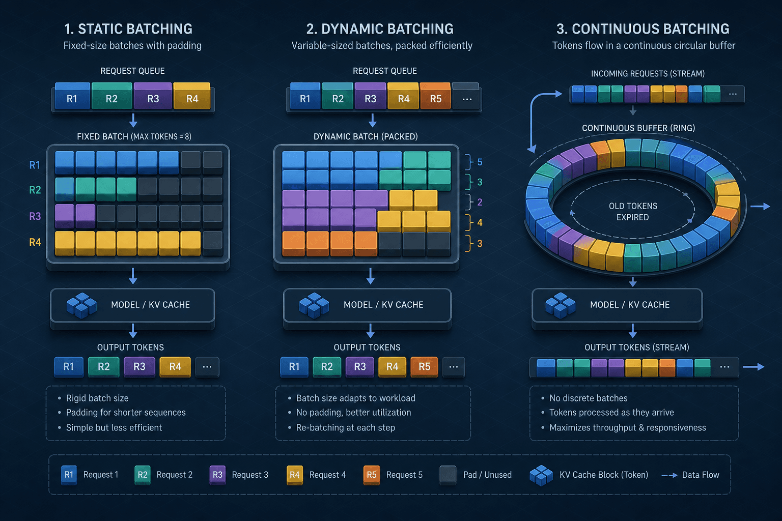
In Large Language Model (LLM) inference, the bottleneck is rarely the sheer number of parameters in the model, but rather the efficiency with which those parameters are processed on the GPU. The primary mechanism for improving throughput is continuous batching: processing multiple requests simultaneously by dynamically managing the lifecycle of each sequence. This article, Part 5 of the LLM Inference from Scratch series, examines the evolution from static to continuous batching, representing a shift from rigid, time-synchronized processing to a fluid, queue-based system that aligns better with the stochastic nature of text generation.

Static Batching: The Lockstep Trap

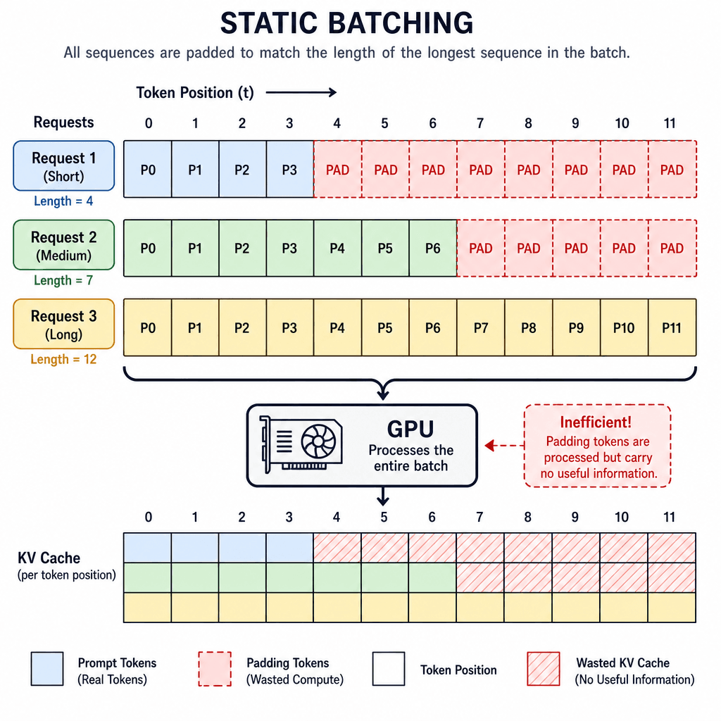
Static batching is the most intuitive approach. A scheduler collects a fixed number of requests, pads them to the same length, and processes them together in a single forward pass.

Consider three requests:

1. "Hello" (2 tokens)
2. "Write a poem about cats" (15 tokens)
3. "Summarize this article..." (50 tokens)

In a static batch of size 3, the system must pad all sequences to the length of the longest one (50 tokens). The GPU processes all three requests in parallel, but for the first 48 tokens of output, the first two requests are effectively doing nothing but processing padding tokens.

The latency of a static batch is determined by the longest sequence in the batch. If a single request has a very long generation length, it holds up the entire batch. This leads to poor GPU utilization because the compute units are idle while waiting for the straggler sequence to finish. Furthermore, static batching requires knowing the maximum sequence length in advance, which is often impossible in production environments where user prompts vary wildly in length.

Dynamic Batching: The Memory-Constrained Compromise

Dynamic batching relaxes the fixed-size constraint. Instead of waiting for a full batch of size $N$, the scheduler adds requests to the batch as long as there is enough GPU memory to hold their Key-Value (KV) caches.

Here, the mechanism shifts from time-synchronization to resource-synchronization. The scheduler maintains a pool of active sequences. When a new request arrives, it is added to the batch if the total KV cache size fits within the GPU's memory budget. However, once a sequence starts generating, it remains in the batch until it completes (either by reaching max tokens, hitting an end-of-sequence token, or timing out).

This improves throughput over static batching because the batch size is adaptive. If many short requests arrive, the batch size grows, saturating the GPU. If long requests arrive, the batch size shrinks, preventing out-of-memory errors.

However, dynamic batching still suffers from the straggler problem. A long-running sequence blocks the GPU resources allocated to it, preventing new short requests from being added to the batch if memory is tight. This creates latency spikes for new users waiting for the system to free up memory from long-running tasks. The trade-off is higher average throughput but unpredictable latency for individual requests.

Continuous Batching: The Queueing Solution

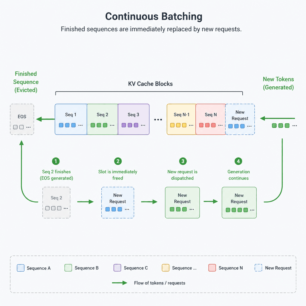
Continuous batching, also known as in-flight batching, fundamentally changes the scheduling granularity. Instead of waiting for an entire batch to finish, the system releases finished sequences immediately and fills the vacated space in the KV cache with new tokens from active sequences.

The mechanism works as follows:

1. Generation Step: The model generates one token for all active sequences in the batch.
2. Completion Check: After each token generation, the scheduler checks which sequences have finished (e.g., reached EOS token).
3. Release and Fill: Finished sequences are removed from the KV cache. Their memory is immediately reassigned to new incoming requests or used to generate additional tokens for remaining active sequences.

This approach treats inference as a continuous stream of token generation rather than discrete batch completions. It maximizes GPU utilization by ensuring that every compute cycle is spent on active, useful work. There is no waiting for the longest sequence to finish; as soon as a sequence completes, its resources are recycled.

Why Continuous Batching Wins

The key advantage of continuous batching is its ability to decouple throughput from latency constraints. In dynamic batching, a long sequence can block the system, causing new requests to queue up. In continuous batching, the system can always accept new requests as long as there is memory, regardless of how long existing sequences are taking. This leads to:

• Higher Throughput: Near 100% GPU utilization because padding is minimized and memory is constantly recycled.
• Lower Latency: New requests are processed as soon as memory is available, without waiting for a full batch to complete.
• Better Resource Efficiency: No wasted cycles on padding tokens for sequences that have already finished.

Implementations like vLLM leverage this by managing the KV cache as a set of blocks, allowing for efficient memory reuse and supporting continuous batching without the overhead of frequent memory allocations. This architectural shift is critical for serving LLMs at scale, where the variability of user input demands a flexible, responsive system.

Conclusion

Static batching is simple but inefficient due to padding and straggler effects. Dynamic batching improves resource utilization but still suffers from latency unpredictability. Continuous batching offers the best of both worlds by treating inference as a continuous queueing process, maximizing throughput while minimizing latency. For ML engineers building production inference systems, understanding this progression is essential for selecting the right infrastructure and optimizing for both cost and user experience.