Tokens, Context Windows, and Why Your Bill Looks Like That

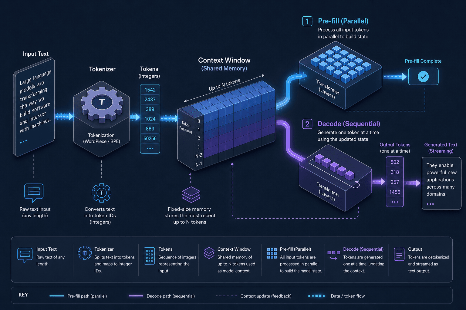
When engineering managers review an LLM infrastructure bill, the first question is rarely "why is it expensive?" but rather "why is it this expensive?" The confusion stems from treating LLM usage as a simple request-response transaction. In reality, it is a two-phase computational process with asymmetric costs. To understand the bill, you must understand the tokenizer, the context window as a memory constraint, and the difference between parallel pre-filling and sequential decoding. All of these factors directly influence the final tokens count that determines your expense.

The Tokenizer: Text to Integers

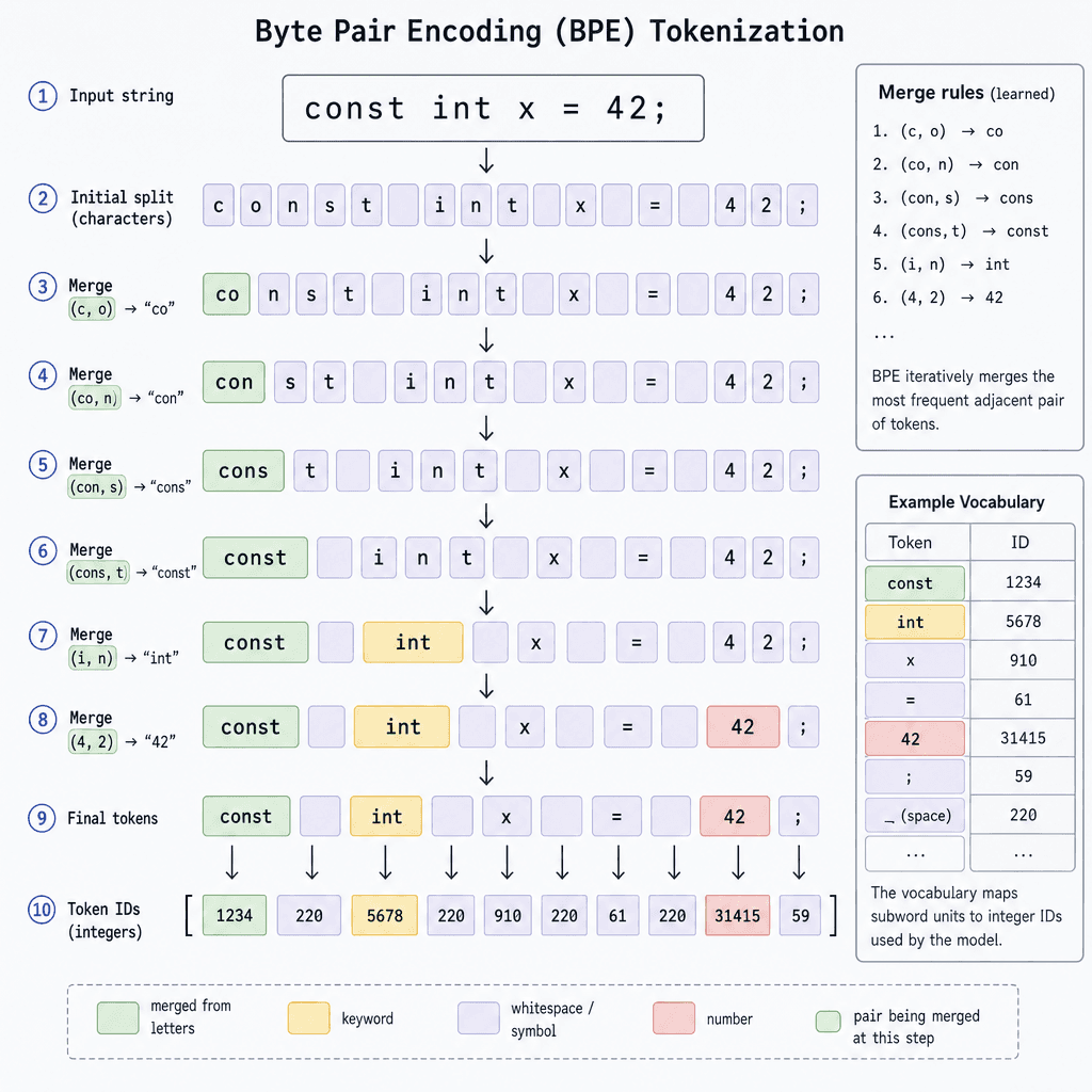
Before any computation occurs, your text must be converted into a format the model can process. This is done by a tokenizer. Most modern LLMs use a variation of Byte Pair Encoding (BPE).

BPE works by breaking text down into subword units. It starts with individual characters and merges the most frequent pairs of characters/subwords into new tokens. This creates a vocabulary where common words (like "the" or "function") are single tokens, while rare words or technical jargon are split into multiple tokens.

Consider a concrete scenario. You pass the string "const int x = 42;" to a standard BPE tokenizer like those used by Llama 2 or GPT-4.

# Pseudocode representation of tokenization
text = "const int x = 42;"
tokens = tokenizer.encode(text)
print(tokens) 
# Output might look like: [1234, 5678, 9012, 3456, 7890]
# Length: 5 tokens

In English, the average ratio is roughly 4 characters per token. However, this efficiency collapses with:

1. Non-Latin scripts: Chinese or Japanese characters often require more tokens per semantic unit.
2. Code: Special characters ({, }, =>) and long variable names are often split.
3. Redundancy: Repetitive phrases do not always compress efficiently if they vary slightly.

Why this matters for your bill: You pay for tokens, not characters. A 10,000-character English prompt might only be 2,500 tokens. A 10,000-character string of minified JavaScript or mixed-language error logs could be 5,000+ tokens. Your bill reflects the token count, which is a lossy compression of your original input. The number of tokens directly dictates the base cost of the request.

The Context Window: Active Working Memory

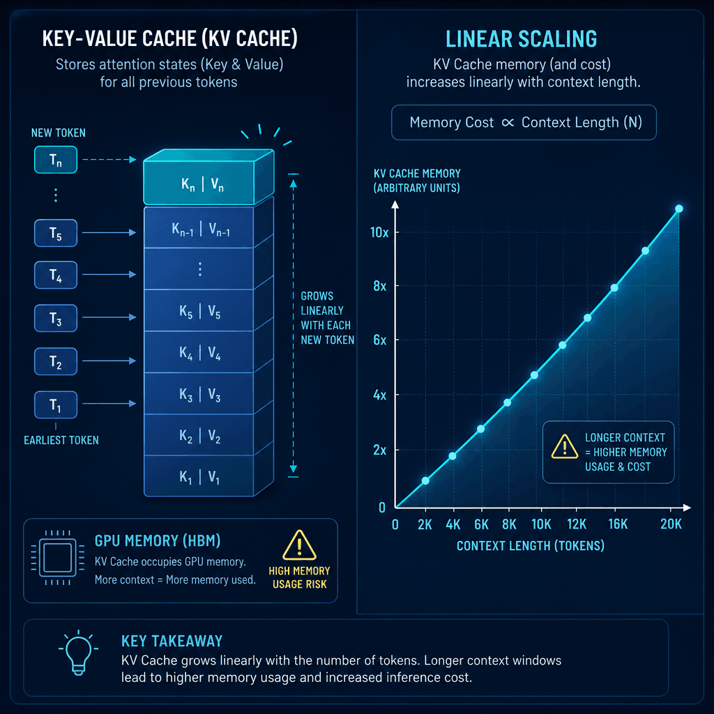
The context window is the maximum number of tokens the model can process in a single interaction. This includes both the input (prompt) and the output (completion).

Crucially, the context window is not just a storage limit; it is the active working memory for the attention mechanism. Every time the model generates a token, it must attend to all previous tokens in the context window to maintain coherence.

This creates a linear scaling problem for memory and compute. If you double the context window, you double the amount of data the model must process for every single token generated. This is managed via the KV Cache (Key-Value Cache), which stores the attention states of previous tokens so they don't need to be recomputed from scratch.

For example, if you have a 100K token context window, the model must keep that entire history in fast GPU memory (HBM) to generate the next word. This is why "long context" models often have higher base prices or stricter rate limits—the hardware footprint is significantly larger, impacting overall llm pricing structures.

Asymmetric Pricing: Input vs. Output

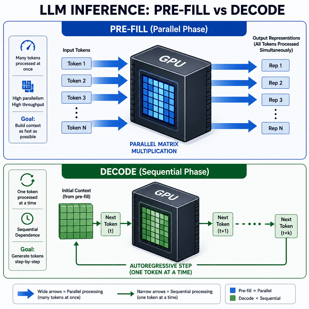
LLM pricing is rarely a flat rate per token. Almost all providers (OpenAI, Anthropic, Google) charge differently for input tokens (prompt) and output tokens (completion).

Input: Parallel Pre-fill

When you send a prompt, the model processes all the tokens in parallel. This is called the pre-fill phase. Because GPUs are excellent at parallel matrix multiplications, this phase is extremely fast and computationally cheap relative to the amount of data processed.

Output: Sequential Decode

When the model generates the response, it does so autoregressively. It predicts one token, then feeds that token back into the model to predict the next, and so on. This is the decode phase.

# Simplified decode loop
for i in range(max_output_tokens):
    # Model attends to ALL previous tokens (input + generated so far)
    # Generates ONE new token
    next_token = model.generate(previous_context)
    previous_context.append(next_token)

This sequential nature makes output generation computationally expensive. The model cannot parallelize across time steps. Therefore, providers charge significantly more per cost per token for outputs (often 2x to 10x the input price) because each output token requires a full forward pass through the entire context history. This disparity is central to understanding llm pricing models.

Why Your Bill Looks Like That

Let's construct a realistic scenario to illustrate the cost drivers.

Scenario: An engineering manager integrates an LLM into a code review tool. The system sends the entire file content (5,000 lines of code) plus a query to the model.

1. Token Count:

   • Input: 5,000 lines of code ≈ 25,000 tokens (due to code verbosity and special characters).
   • Output: The model generates a 500-word review ≈ 700 tokens.
   • Total Context: 25,700 tokens.

2. Cost Calculation (using hypothetical $1/M input, $3/M output pricing):

   • Input Cost: 25,000 * $1 / 1,000,000 = $0.025
   • Output Cost: 700 * $3 / 1,000,000 = $0.0021
   • Total: $0.0271

At first glance, the input cost dominates. However, consider the latency. The pre-fill phase (input) might take 0.1 seconds. The decode phase (output) takes 2.0 seconds. The user experiences the latency of the output.

Now, consider scaling. If you increase the file size to 50,000 lines:

• Input tokens: 250,000.
• Output tokens: 700 (assuming the review length doesn't scale linearly with file size, though it might).
• Input Cost: $0.25.
• Output Cost: $0.0021.

The input cost scales linearly with your data volume. The output cost remains relatively stable if the response length is bounded. This is why bills for data-heavy applications (like summarizing large logs or processing entire repositories) explode: you are paying for the massive pre-fill phase, which is cheap per cost per token but expensive in aggregate volume.

Optimizing for Cost

Understanding these mechanisms allows for targeted optimization in any llm pricing strategy:

1. Reduce Input Tokens: Use more efficient tokenizers. Prune irrelevant context from the prompt. Use compression techniques like summarization before sending to the main model.
2. Cap Output Tokens: Set strict max_tokens limits. Use structured output formats (JSON) to ensure predictable lengths.
3. Cache Context: If you send the same system prompt or large static context repeatedly, use prompt caching features (available in some provider APIs) to avoid re-computing the pre-fill for unchanged prefixes.

Conclusion

Your LLM bill is a reflection of computational asymmetry. Input tokens are cheap, parallel, and represent the "setup" cost. Output tokens are expensive, sequential, and represent the "work" cost. The context window is the constraint that binds them together, growing linearly in memory and compute requirements. By optimizing token counts and understanding the pre-fill/decode divide, you can bring these cost drivers under control.