The KV Cache Explained Without the Math

When you ask a Large Language Model (LLM) like Llama or GPT to write an email, it doesn’t generate the whole email at once. It generates it one word at a time, a process called autoregressive generation. You type the prompt, the model predicts the first token, then you feed that token back in to predict the second, and so on.

This is Part 4 of the LLM Inference from Scratch series.

At first glance, this seems inefficient. Why does the model need to "remember" the previous words every single time it predicts the next one? Why can’t it just look at the current word and spit out the next?

The answer lies in how the Transformer architecture works, specifically the Attention Mechanism. To understand the KV cache, we first need to understand why the model is so obsessed with looking back at the entire history.

The Problem: Rereading the Book

Imagine you are reading a thick novel. You are on page 100. To understand the sentence on page 100, you might need to recall character details from page 10. But you don’t need to reread pages 1 through 99 to understand page 100. You just need the relevant snippets.

In a naive LLM inference scenario, the model acts like a reader who has never read the book before. Every time it tries to generate the next word, it takes the entire prompt plus all previously generated words and re-analyzes them from scratch. This redundancy is why the KV cache, often referred to as the attention cache, is such a critical optimization.

If your prompt is 1,000 tokens long, and the model generates 1,000 more tokens, here is what happens:

1. To generate token 1, it attends to 1,000 tokens.
2. To generate token 2, it attends to 1,001 tokens.
3. To generate token 100, it attends to 1,099 tokens.

This creates a quadratic bottleneck. As the conversation gets longer, the computation required to generate the next word grows linearly with the total length. For long contexts, this becomes prohibitively slow. The GPU spends most of its time doing the same math over and over again, calculating how token B relates to token A, even though that relationship hasn’t changed since the first step.

The Solution: The KV Cache

The KV cache solves this by recognizing a simple fact: the relationship between previous tokens never changes.

Once the model has processed the initial prompt, the "meaning" of the first token in relation to the second token is fixed. It doesn’t matter if you are generating the 100th word or the 1,000th word; the context provided by the first 100 words remains identical.

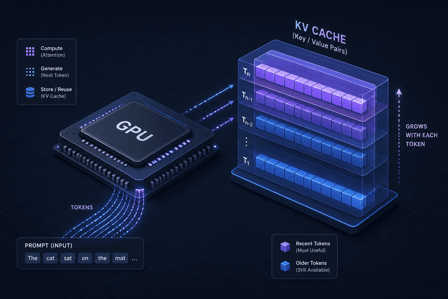
Instead of recalculating this context, the model stores it. This stored context is the KV Cache.

What are K and V?

In the attention mechanism, every token is converted into three vectors:

1. Query (Q): "What am I looking for?"
2. Key (K): "What do I contain?" (Like an index card label).
3. Value (V): "Here is the actual content associated with this key." (Like the text on the index card).

When the model looks at a new token (the Query), it compares its Query vector against the Key vectors of all previous tokens. If there’s a match, it pulls the corresponding Value vectors to help predict the next word.

The KV cache simply stores the Keys and Values of all previously processed tokens.

1. Initial Prompt: The model processes the user's input. It calculates the Q, K, and V vectors for every token in the prompt.
2. Cache Storage: Queries are transient and computed per-step for the new token, whereas Keys and Values are persistent across steps. Therefore, the model discards the current step's Queries but saves the K and V vectors in GPU memory.
3. Generation Step: When generating the next token, the model only calculates the Q, K, and V for that single new token.
4. Attention Lookup: Instead of calculating K and V for the whole history, it fetches the pre-computed K and V vectors from the cache. It then performs the attention calculation using only the new Query against the old Keys.

This reduces the per-token generation complexity from O(N^2) to O(N) by caching previous keys and values, avoiding redundant attention calculations for the history. The attention calculation still scales linearly with the number of cached tokens, but we avoid re-processing the entire sequence.

The Trade-off: Memory vs. Compute

The KV cache is a classic space-time trade-off. We are swapping GPU memory for GPU compute.

Because the cache stores a vector for every token in the conversation, its size grows linearly with the sequence length. For a typical model, the KV cache might take up several gigabytes of VRAM for a single conversation.

This has a direct impact on concurrency—how many users you can serve simultaneously.

Scenario A: No KV Cache

If you didn’t use a cache, you would use very little memory per request (just the current token's vectors), but the GPU would be maxed out doing redundant math. You could fit thousands of requests in memory, but each request would take forever to process.

Scenario B: With KV Cache

With the cache, each request consumes significant VRAM. If you have a GPU with 80GB of VRAM, and each request’s KV cache grows to 5GB, you can only serve 16 concurrent requests. If you try to serve 20, the GPU will run out of memory (OOM), and the extra requests will have to wait.

However, the upside is speed. Because the GPU isn’t wasting cycles on redundant math, those 16 requests generate tokens much faster. The latency per token drops dramatically.

How This Enables Batch Inference

The KV cache is the reason modern LLM inference engines (like vLLM, TGI, or TensorRT-LLM) can handle batched inference efficiently.

When you batch 10 requests together, the GPU processes them in parallel. Without a KV cache, the GPU would have to run the full attention mechanism for all 10 requests, re-attending to the full history for each one. This is computationally expensive and often inefficient due to padding (short requests waiting for long requests).

With a KV cache:

1. The GPU allocates a contiguous block of memory for the KV cache of all 10 requests.
2. During the prefill phase (processing the initial prompt), it computes and stores the K/V vectors for all 10 prompts.
3. During the decode phase (generating tokens), it only computes the attention for the new tokens of all 10 requests, fetching their respective cached K/V vectors.

This allows the GPU’s tensor cores to work on many different requests simultaneously without redundant computation. The bottleneck shifts from "how much math can we do?" to "how much memory can we hold?"

Conclusion

The KV cache is not a magic algorithm; it is a data structure optimization. It acknowledges that in autoregressive generation, the past is static. By storing the Keys and Values of the past, we avoid recomputing them, turning an expensive, history-dependent operation into a cheap, lookup-based operation.

This optimization is critical for making LLMs usable. Without it, generating a simple response would require seconds of redundant computation. With it, we get sub-second latency, at the cost of increased VRAM usage. Understanding this trade-off is essential for anyone deploying LLMs, as it dictates how you size your GPUs, how many users you can support, and how you manage memory fragmentation.

See the vLLM paper and Hugging Face’s implementation guides for deeper technical details on the memory layout and paged attention optimizations used in production systems.