Estimating LLM Costs Before You Build

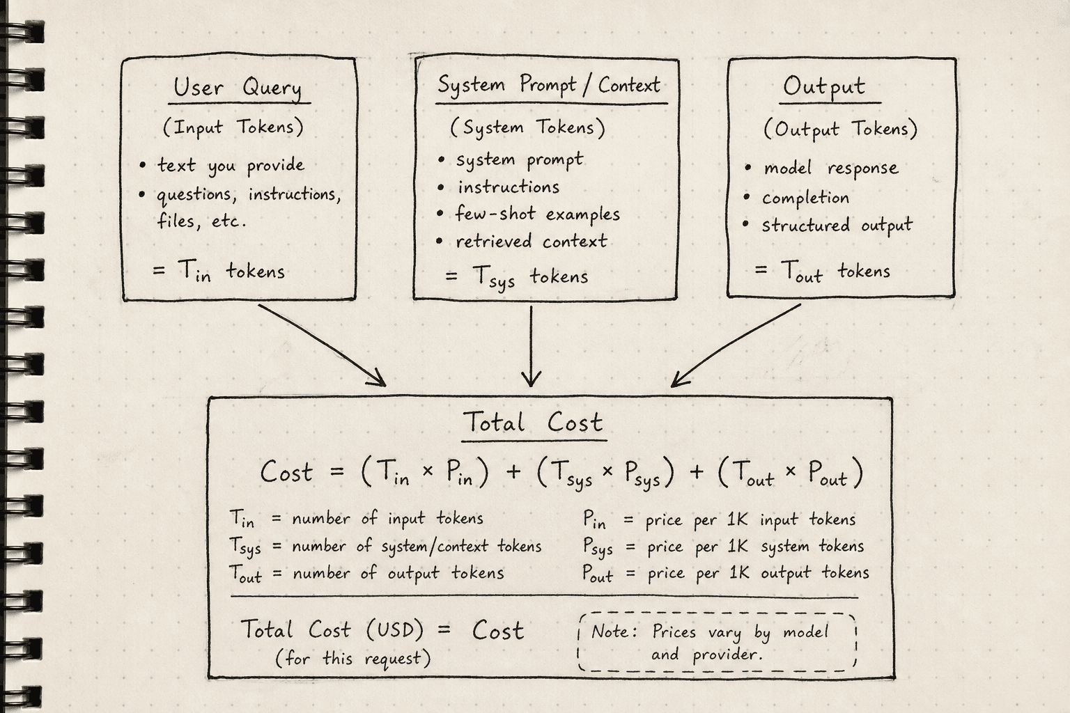
Most engineering managers treat Large Language Model (LLM) costs as a linear function of user requests. If you have 1,000 users and each makes one request, the cost is $1,000 \times \text{price\_per\_request}$. This mental model is fundamentally broken. LLMs are not stateless web endpoints; they are compute-intensive inference engines where cost is driven by token throughput, context window utilization, and caching efficiency. To build within budget, you must shift from tracking "requests" to tracking "tokens" and "cache hits."

This guide outlines the mechanism of LLM unit economics, how to forecast token consumption using workflow mapping, and how to apply sensitivity analysis to protect your budget against variance.

The Unit Economics of Tokens

The fundamental unit of LLM billing is the token. A token is a subword unit, typically representing 0.75 words on average, but this ratio varies wildly by language and domain. The critical insight for architects is that the "input" and "output" are billed separately, and the input size is often orders of magnitude larger than the visible user query.

When a user sends a prompt, the system does not just tokenize that string. It constructs a payload containing:

1. User Query: The actual text.
2. System Prompt: Hidden instructions defining the AI's behavior.
3. History: Previous turns in the conversation.
4. Tool Definitions: JSON schemas for available functions.

If you estimate cost based only on the user query, you will underestimate input costs by 20–50% in typical chat applications. The mechanism here is straightforward: every byte sent to the model’s context window is processed by the GPU. The cost is $(\text{Input Tokens} \times \text{Price Per Input Token}) + (\text{Output Tokens} \times \text{Price Per Output Token})$.

Token Forecasting via Workflow Mapping

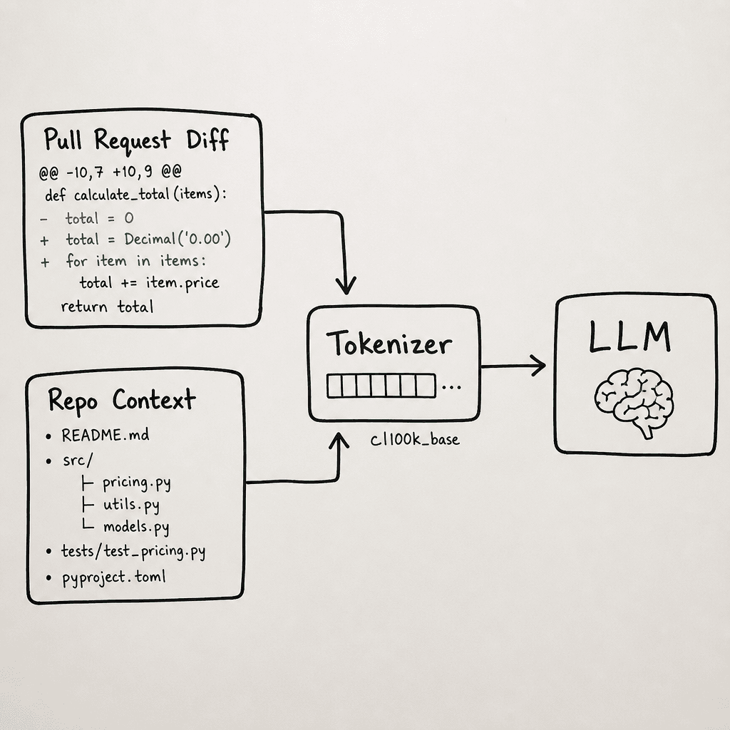
Abstract volume estimates ("10k requests/day") are useless for budgeting. You need a precise token forecast derived from workflow mapping. Let’s use a concrete scenario: a Code Review Bot that analyzes pull requests and returns a summary.

Step 1: Map the Artifact Sizes

Identify the named artifacts involved in each request. In our Code Review Bot, the artifacts are:

• diff_text: The code changes (variable size).
• repo_context: Relevant file headers or previous PR comments (fixed size).
• system_prompt: The review guidelines (fixed size, ~500 tokens).

Step 2: Calculate Token Counts

Use a standard tokenizer model (like cl100k_base used by GPT-4) to estimate token counts. Do not guess. Write a small script to tokenize representative samples.

Component	Avg Characters	Est. Tokens	Notes
System Prompt	3,000	2,500	Fixed overhead
Repo Context	5,000	4,000	Fixed overhead
Diff Text (Small)	2,000	1,800	Low variance
Diff Text (Large)	20,000	18,000	High variance
Output Summary	500 chars	400	Generation cost

Step 3: Sum the Effective Input

For a small diff, the total input tokens are $2,500 + 4,000 + 1,800 = 8,300$ tokens. For a large diff, it is $2,500 + 4,000 + 18,000 = 24,500$ tokens.

If you have 1,000 daily reviews, with 80% small diffs and 20% large diffs:

• Small: $800 \times 8,300 = 6,640,000$ input tokens.
• Large: $200 \times 24,500 = 4,900,000$ input tokens.
• Total Input: $11,540,000$ tokens.
• Total Output: $1,000 \times 400 = 400,000$ tokens.

At current OpenAI GPT-4o pricing ($2.50/$10 per 1M tokens), the daily cost is:

$(11.54 \times 2.50) + (0.4 \times 10.00) = \$28.85 + \$4.00 = \$32.85$/day.

Without mapping the artifacts, you might have estimated based on a "500-token prompt," leading to a forecast of ~$1.50/day—a 20x error.

The Caching Multiplier

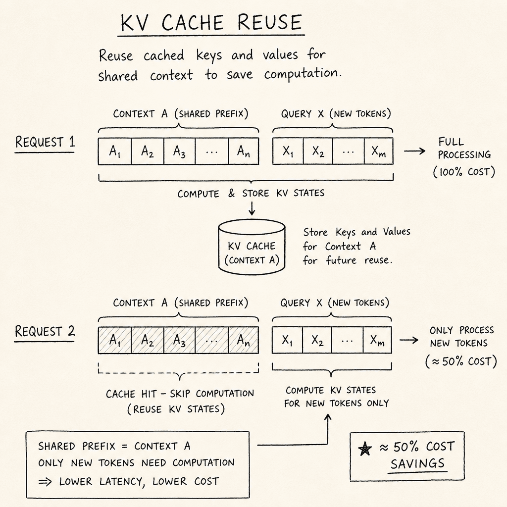
The most significant lever for reducing LLM costs is prefix caching (or KV cache reuse). Modern serving engines like vLLM or TGI (Text Generation Inference) store the key-value (KV) pairs of the prompt in memory. If a subsequent request has a matching prefix (e.g., the same system prompt and repo context), the engine skips recomputing those tokens.

The mechanism works as follows:

1. Request 1 arrives with Context A + Query X. The engine computes KV cache for A and X. Cost: Full price for A + X.
2. Request 2 arrives with Context A + Query Y. The engine finds Cache A. It only computes KV cache for Y. Cost: Discounted price for Y (often 10–50% of full input price).

Your token forecast must include a Cache Hit Rate (CHR). In a code review bot, the system_prompt and repo_context are identical for many requests. If 70% of your requests share the same context, your effective input cost drops significantly.

A realistic model looks like this:

• Non-Cached Inputs: $10\%$ of requests (unique contexts).
• Cached Inputs: $90\%$ of requests (reused contexts).

If the cached input price is 50% of the full input price (a conservative estimate), the weighted average input cost becomes:

$(0.10 \times 1.0) + (0.90 \times 0.5) = 0.55$ times the full price.

This halves your input cost forecast. Ignoring caching is the single most common error in LLM budgeting.

Sensitivity Analysis for Budgeting

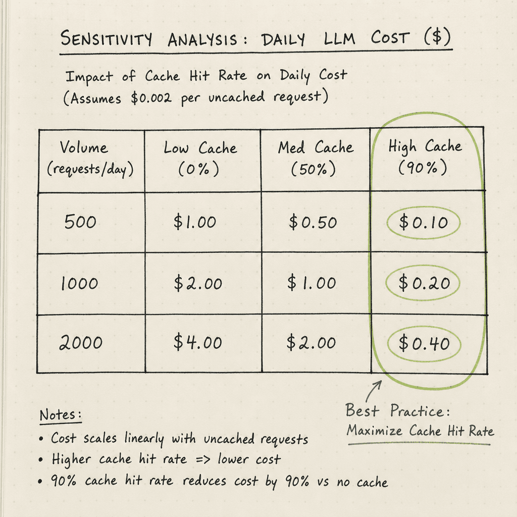
No token forecast is perfect. Token counts vary, cache hit rates fluctuate, and model prices change. You must build a sensitivity analysis to understand the range of possible costs.

Define three variables:

1. Avg Input Tokens ($I$): Range from 8k to 25k.
2. Cache Hit Rate ($C$): Range from 0% (no caching) to 90% (highly repetitive).
3. Daily Volume ($V$): Range from 500 to 2,000 requests.

Create a simple spreadsheet or script to calculate cost across these dimensions. Identify the Break-Even Point where your budget is exceeded.

Example Sensitivity Table (Daily Cost):

Volume	Low Cache (0%)	Med Cache (50%)	High Cache (90%)
500 reqs	$15.00	$7.50	$4.50
1,000 reqs	$30.00	$15.00	$9.00
2,000 reqs	$60.00	$30.00	$18.00

This table reveals that caching is more impactful than volume scaling. Doubling volume with high caching costs less than halving volume with no caching. This insight directs your engineering effort: prioritize implementing efficient caching layers (e.g., Redis-backed prompt caching or vLLM prefix caching) over simply optimizing code.

Conclusion

Accurate LLM cost estimation is an exercise in tracing data flow. You must:

1. Map artifacts: Measure the true size of inputs, including hidden context.
2. Model caching: Apply a realistic hit rate to reduce effective input costs.
3. Stress test: Use sensitivity analysis to find the cost drivers.

By treating tokens as the unit of currency and caching as a discount mechanism, you move from guessing to engineering. This approach allows you to predict costs within 10–20% accuracy, enabling reliable budgeting for AI infrastructure.