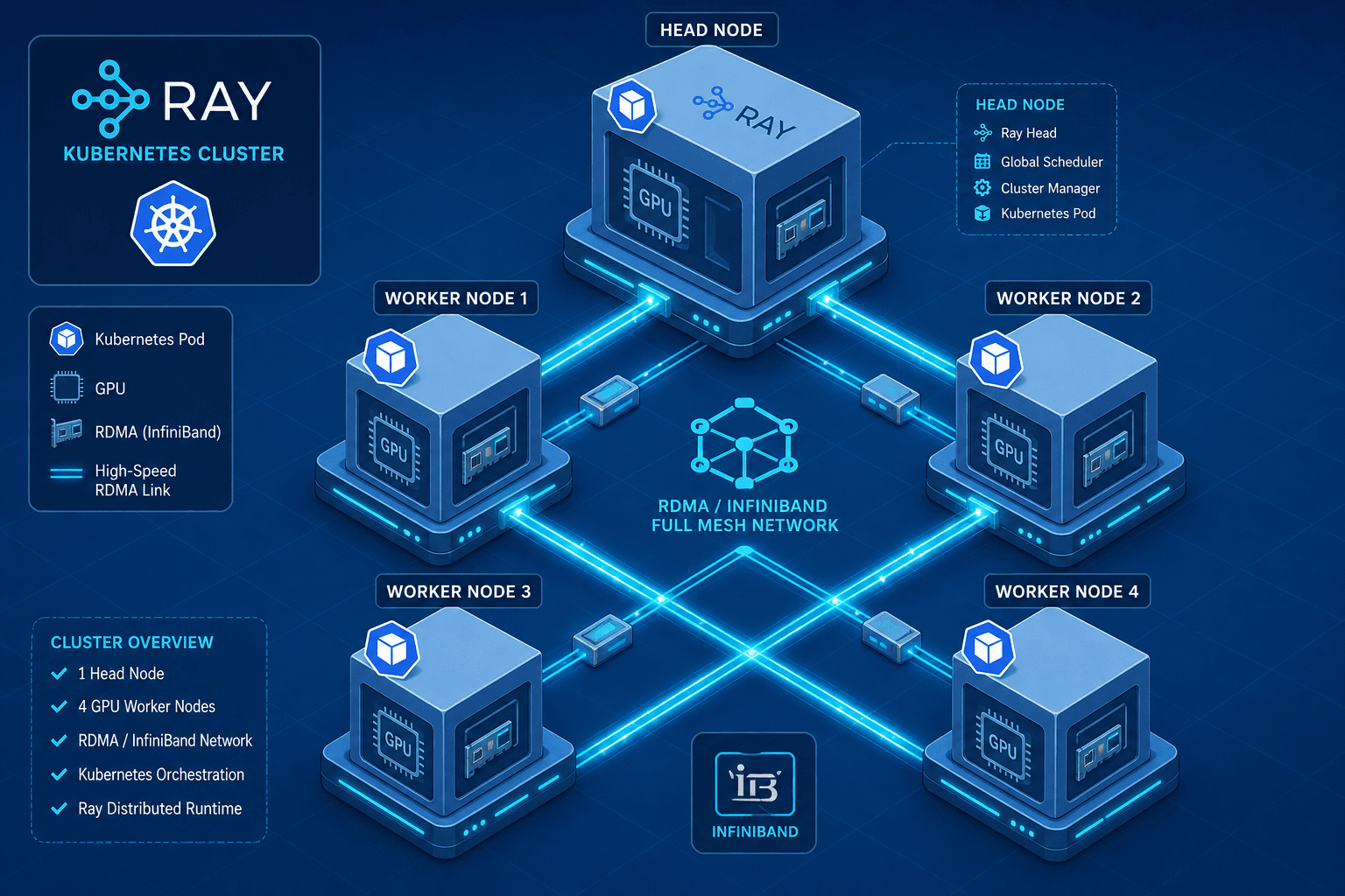
Multi-Node Inference with Ray and Kubernetes

Deploying Large Language Models (LLMs) across multiple nodes transforms inference from a simple scaling problem into a complex distributed systems challenge. When you move beyond a single GPU, you introduce network latency, synchronization overhead, and resource fragmentation. Most engineers attempt to scale by simply adding more Kubernetes replicas, but this fails because standard Kubernetes schedulers treat pods as independent entities. In a multi-node Ray cluster, if one node is delayed by even a few seconds, the entire inference pipeline stalls due to synchronization barriers.

This guide explains the mechanism-level requirements for running Ray Serve on Kubernetes: gang scheduling to ensure atomic resource allocation and RDMA integration to minimize inter-node communication latency.

The Synchronization Bottleneck

In a single-node setup, Ray actors communicate via shared memory or local IPC, which operates at nanosecond to microsecond latencies. In a multi-node setup, these messages travel over the network. If Node A starts its Ray head and worker before Node B, Node A begins processing requests that require data from Node B. Node B is not ready. Node A blocks. This is known as the "straggler problem."

Standard Kubernetes scheduling does not solve this. The default scheduler places Pod A, then Pod B, then Pod C. If Pod C is delayed due to node pressure or image pull time, Pods A and B are left waiting. For distributed inference, where all nodes must participate in every request (e.g., tensor parallelism or pipeline parallelism), this partial startup is catastrophic.

Configuring ray serve kubernetes effectively requires addressing this synchronization issue at the infrastructure level, rather than attempting to handle it through application-level retries or timeouts.

Gang Scheduling: Atomic Resource Allocation

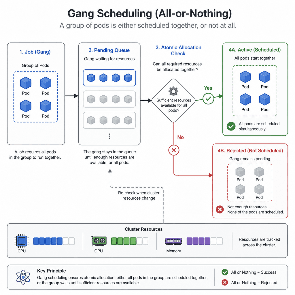
Gang scheduling solves this by treating a group of pods as a single scheduling unit. The scheduler evaluates the entire group against cluster capacity. If the cluster cannot satisfy the resource requirements for all pods in the group simultaneously, the scheduler rejects the entire group. This ensures that when a Ray cluster starts, every node is available at the same time.

Implementing gang scheduling in Kubernetes typically involves a custom scheduler extension, such as Volcano or Kueue. These schedulers introduce the concept of a "job" that contains multiple pods. The scheduler maintains a queue of jobs and only dispatches them when the global resource constraints are met for the entire job.

For Ray, this means configuring the Ray operator to request scheduling via these gang-aware schedulers. The Ray head pod and all worker pods are grouped into a single gang. The mechanism works as follows:

1. The Ray operator submits a Job object to the gang scheduler.
2. The gang scheduler checks if the cluster has enough CPU, GPU, and memory for all pods in the Job.
3. If yes, all pods are bound to nodes simultaneously.
4. If no, the Job remains pending until resources are freed.

This eliminates the race condition where nodes start at different times. It also prevents resource fragmentation, where small gaps in resource availability prevent large workloads from starting, even if the total cluster capacity is sufficient. When combined with rdma networking, gang scheduling ensures that both compute and communication resources are allocated atomically, preventing scenarios where nodes have GPUs but lack the high-speed network connectivity required for synchronized execution.

High-Speed Networking: RDMA vs. TCP/IP

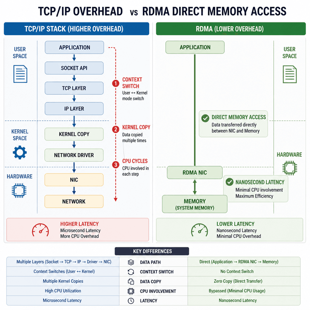
Once nodes are synchronized, the next bottleneck is network throughput. Standard Kubernetes networking uses TCP/IP over Ethernet, which involves multiple context switches and kernel copies. For LLM inference, where tensors are large and communication frequency is high, this overhead introduces significant latency.

Remote Direct Memory Access (RDMA) allows one node to read or write memory directly from another node's memory without involving the CPU or operating system kernel. This reduces latency from milliseconds to microseconds and frees up CPU cycles for model computation.

Ray supports RDMA indirectly through NCCL, the underlying communication library used for its collective operations. To enable this, you must:

1. Hardware Setup: Ensure nodes have InfiniBand or RoCE (RDMA over Converged Ethernet) adapters.
2. Kernel Bypass: Configure the network interface to use user-space RDMA libraries (e.g., libibverbs for InfiniBand).
3. Ray Configuration: Specify the correct network interface in the Ray cluster configuration.

In a Kubernetes environment, enabling RDMA requires special handling. Standard CNI (Container Network Interface) plugins do not support RDMA natively. rdma networking requires special handling because SR-IOV or DPDK integrations are often needed to expose hardware capabilities to containers. SR-IOV allows a single physical NIC to appear as multiple virtual functions, each assignable to a pod. This gives each Ray worker direct access to the hardware.

The mechanism for RDMA in Ray involves creating a dedicated network interface for Ray's internal communication. This interface is isolated from the Kubernetes overlay network (e.g., Calico or Cilium) to avoid packet encapsulation overhead. Ray uses this interface for all-reduce operations, which are critical for aggregating gradients in distributed training and for load balancing in distributed inference. For distributed llm serving, minimizing this latency is crucial to maintaining high throughput and low time-to-first-token.

Operational Walkthrough: Deploying Ray Serve

Let's look at a concrete example of deploying a multi-node Ray Serve cluster on Kubernetes with gang scheduling and RDMA considerations. This setup is fundamental for distributed llm serving at scale.

First, ensure your Kubernetes cluster has a gang scheduler installed. For this example, we assume Volcano is configured as the default scheduler for certain namespaces.

apiVersion: ray.io/v1
kind: RayCluster
metadata:
  name: ray-cluster-inference
  annotations:
    # Request gang scheduling via Volcano
    volcano.sh/queue-name: high-priority-queue
spec:
  rayVersion: '2.9.0'
  headGroupSpec:
    rayStartParams:
      dashboard-host: '0.0.0.0'
      num-cpus: '0'
      num-gpus: '0'
    template:
      spec:
        schedulerName: volcano # Explicitly use Volcano scheduler
        containers:
        - name: ray-head
          image: rayproject/ray:2.9.0
          resources:
            limits:
              cpu: "4"
              memory: "16Gi"
              nvidia.com/gpu: "0" # Head node doesn't need GPU for serving
          env:
          - name: RAY_DEDUP_LOGS
            value: "0"
          - name: RAY_GRAFANA_HOST
            value: "http://grafana.monitoring.svc.cluster.local:3000"
  workerGroupSpecs:
  - groupName: gpu-workers
    replicas: 4
    minReplicas: 4
    maxReplicas: 4
    rayStartParams:
      num-cpus: "0"
      num-gpus: "1"
      resources: '{"custom_resource": 1}'
    template:
      spec:
        schedulerName: volcano
        # Enable RDMA if supported by your CNI
        hostNetwork: true 
        dnsPolicy: Default
        containers:
        - name: ray-worker
          image: rayproject/ray:2.9.0-gpu
          resources:
            limits:
              cpu: "8"
              memory: "32Gi"
              nvidia.com/gpu: "1"
              # Request SR-IOV VF if using RDMA
              intel.com/sriov_net: "1"
          env:
          - name: RAY_DEDUP_LOGS
            value: "0"
          - name: NCCL_SOCKET_IFNAME
            value: "ib0" # InfiniBand interface

In this manifest, several key mechanisms are at play:

1. Scheduler Name: The schedulerName: volcano annotation ensures that the pods are scheduled by the gang scheduler, not the default K8s scheduler. This guarantees that all four worker pods and the head pod are placed simultaneously.
2. Resource Limits: The nvidia.com/gpu: "1" limit ensures that each worker gets exactly one GPU. The gang scheduler will not place a worker unless a GPU is available on the target node.
3. Network Interface: The NCCL_SOCKET_IFNAME environment variable tells the underlying NCCL communication library to use the InfiniBand interface (ib0) for internal communication. This bypasses the Kubernetes overlay network.
4. Host Network and DNS: Using hostNetwork: true allows Ray to bind directly to the host's network interfaces, which is often required for RDMA to function correctly. We set dnsPolicy: Default to avoid conflicts with the Kubernetes cluster DNS when using host networking, ensuring that external DNS resolution works as expected while the data plane traffic bypasses the overlay. Note that if cluster-internal service discovery is strictly required, ClusterFirstWithHostNet may be used with careful CNI configuration, but Default is safer for pure RDMA setups relying on static hostnames or external DNS.

Conclusion

Multi-node inference on Kubernetes is not just about adding more nodes; it is about synchronizing them. Gang scheduling ensures that all nodes start together, eliminating stragglers caused by asynchronous startup. RDMA integration reduces the latency of inter-node communication, allowing the cluster to scale efficiently.

By combining these mechanisms, you create a stable foundation for distributed llm serving. The key takeaway is that Kubernetes alone is not enough. You need specialized schedulers and network configurations to handle the unique demands of distributed AI workloads. As models grow larger and more complex, these infrastructure details will become the primary determinant of performance and cost efficiency.