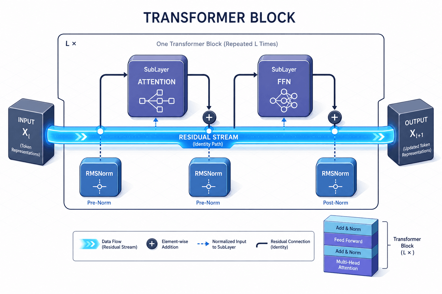
Normalization and Residual Streams: Stabilizing Transformer Training

Normalization and Residual Streams

In the transformer architecture, the residual stream acts as the central artery for information flow, carrying accumulated token representations through successive layers of attention and feed-forward networks. However, this design introduces a fundamental mechanical challenge: without intervention, activation magnitudes in the residual streams grow without bound as depth increases. This growth leads to numerical instability, saturating activation functions and breaking gradient flow. Normalization layers—specifically layernorm and rmsnorm—are not merely optional regularizers; they are essential mechanisms that constrain the variance of the residual stream, ensuring that the signal remains within a computable range for downstream operations. This deep-learning challenge requires careful normalization.

The Residual Stream Variance Problem

To understand why normalization is required, we must examine the mechanics of the residual connection. A typical Transformer block updates the hidden state $x$ by adding the output of a sub-layer (e.g., attention or feed-forward network) to the input:

$x_{new} = x_{old} + \text{SubLayer}(x_{old})$

If we trace this operation through $L$ layers, the final representation is the sum of the initial embedding and the outputs of all $L$ sub-layers. Assuming the outputs of these sub-layers have non-zero mean and variance, the variance of the sum grows linearly with the number of layers. In practice, because neural network weights are initialized to have small variances, the initial outputs are small. However, as training progresses, weights adjust, and the magnitude of these residual updates accumulates.

Without normalization, the activations in the residual stream can grow to extremely large values. Most activation functions used in modern Transformers, such as GELU (Gaussian Error Linear Unit) or SiLU (Sigmoid Linear Unit), have saturating gradients for extreme inputs. When the input to GELU is very negative, the gradient approaches zero. This is known as the "saturation problem." If the residual stream grows too large, the gradients flowing backward through the network vanish, stopping learning. Conversely, if the values oscillate wildly, gradients explode. Normalization fixes this by forcing the activations into a consistent statistical distribution.

LayerNorm: Stabilizing Per-Token Activations

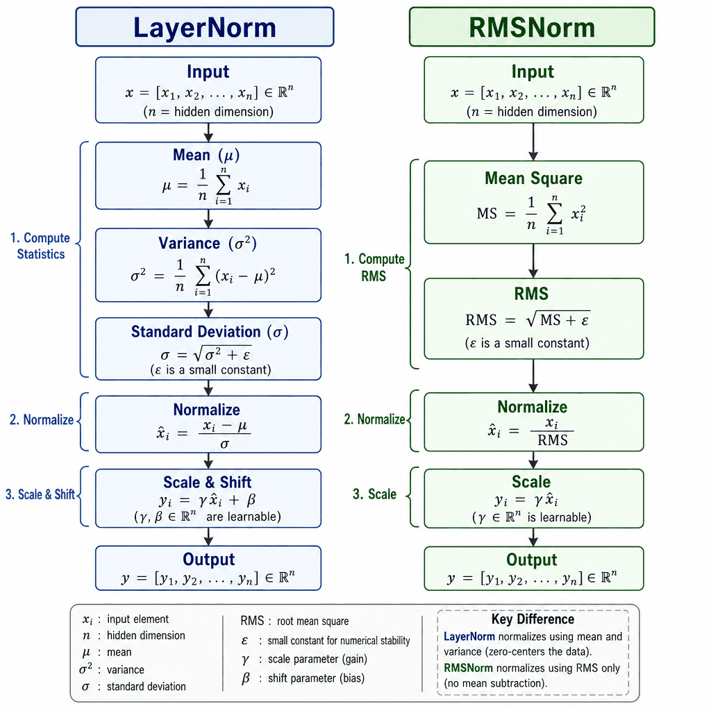
Layer Normalization (layernorm) was introduced to address the instability of batch-dependent statistics in variable-length sequences. Unlike BatchNorm, which normalizes across the batch dimension, layernorm normalizes across the feature dimensions for each individual token. This is crucial because the semantic meaning of a token is contained within its feature vector, not its position relative to other tokens in the batch.

The mechanism of layernorm involves two steps: centering and scaling. For a given token's activation vector $h$ with dimension $d$, layernorm computes the mean $\mu$ and variance $\sigma^2$ across the $d$ dimensions:

$\mu = \frac{1}{d} \sum_{i=1}^{d} h_i$ $\sigma^2 = \frac{1}{d} \sum_{i=1}^{d} (h_i - \mu)^2$

It then normalizes the vector:

$\hat{h}_i = \frac{h_i - \mu}{\sqrt{\sigma^2 + \epsilon}}$

Finally, it applies a learnable scale parameter $\gamma$ and shift parameter $\beta$:

$y_i = \gamma \hat{h}_i + \beta$

This process ensures that regardless of the depth of the network, the activations entering the next sub-layer have a mean of approximately 0 and a variance of approximately 1. This keeps the inputs to activation functions like GELU in their most sensitive region, where gradients are strongest. The parameters $\gamma$ and $\beta$ allow the network to recover any necessary scaling or shifting that normalization might have removed, preserving the representational capacity of the model.

RMSNorm: Removing the Mean

While layernorm is effective, rmsnorm simplifies this by removing the mean subtraction step.

Proposed by Zhang and Sennrich (2019), rmsnorm assumes that centering the data (subtracting the mean) is less critical for stability than scaling the variance. The RMS value of a vector $h$ is calculated as:

$\text{RMS}(h) = \sqrt{\frac{1}{d} \sum_{i=1}^{d} h_i^2}$

The normalized output is then:

$\hat{h}_i = \frac{h_i}{\text{RMS}(h)} \cdot \gamma_i + \beta_i$

(Note: $\beta$ is often omitted in rmsnorm implementations as it is redundant when the mean is already zero, but some variants include it for flexibility).

By skipping the mean calculation, rmsnorm reduces the computational overhead and memory access patterns. Empirical studies show that rmsnorm performs comparably to LayerNorm in terms of training stability and final model performance, while being faster to compute. This makes it the preferred choice in many modern large language models, such as LLaMA.

Pre-Norm: Strategic Placement for Gradient Stability

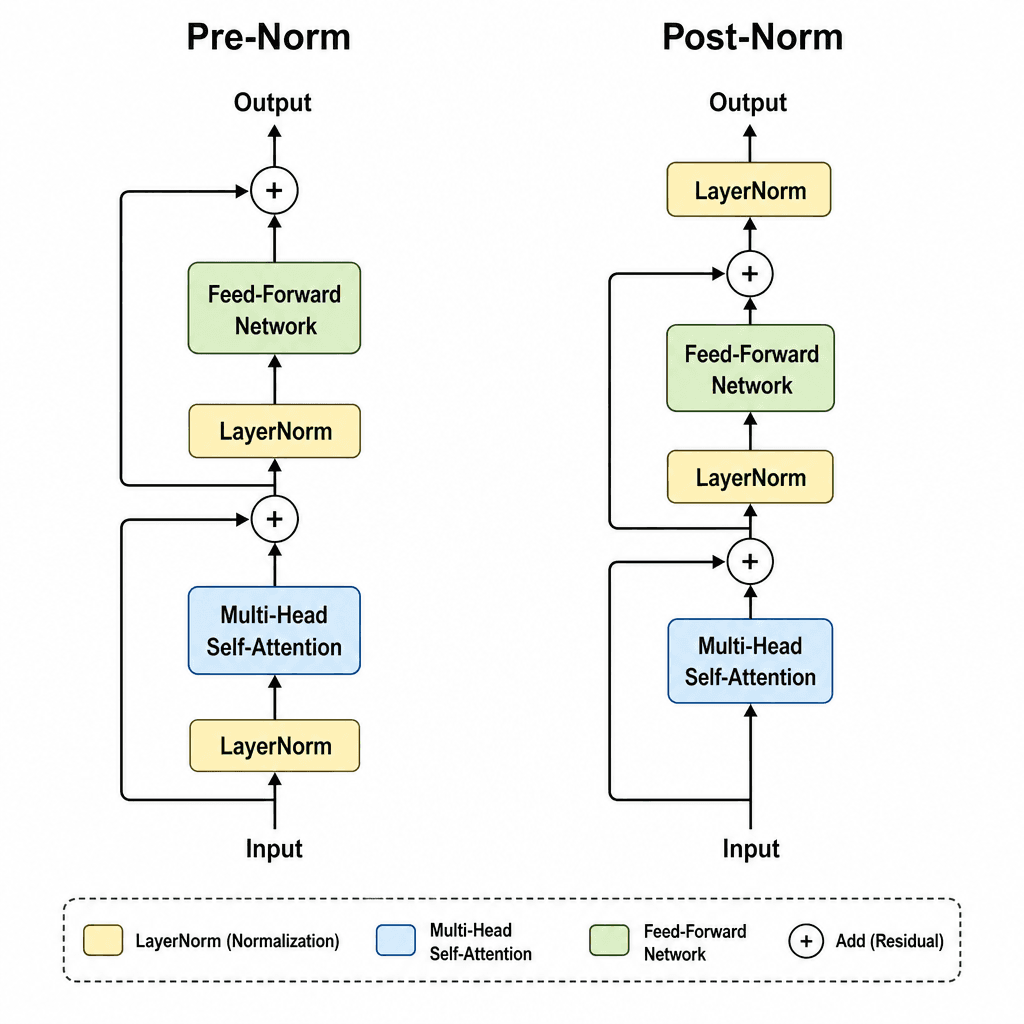
The location of the normalization layer within the Transformer block is just as important as the normalization algorithm itself. There are two primary strategies: post-norm and pre-norm.

In Post-Norm, the normalization is applied after the sub-layer:

$x_{new} = \text{LayerNorm}(x_{old} + \text{SubLayer}(x_{old}))$

In Pre-Norm, the normalization is applied before the sub-layer:

$x_{new} = x_{old} + \text{SubLayer}(\text{LayerNorm}(x_{old}))$

For deep Transformer models, Pre-Norm is generally superior for training stability. This was highlighted by Xiong et al. (2020), who demonstrated that Post-Norm suffers from vanishing gradients in very deep networks. In Post-Norm, the residual connection adds the original input $x_{old}$ to the normalized output. As the network deepens, the gradient of the loss with respect to the input of a layer involves the product of many Jacobians from the sub-layers. If these Jacobians have norms less than 1, the gradient vanishes.

Pre-Norm changes this dynamic. By normalizing the input before it enters the sub-layer, the scale of the activations is controlled at every step, preventing saturation in the attention and feed-forward components. This ensures that the gradients flowing backward do not get attenuated as severely. Furthermore, the unnormalized residual path in Pre-Norm helps preserve gradient magnitude more effectively than Post-Norm, where the residual path is also normalized, allowing the model to bypass the sub-layer entirely if the identity mapping is optimal.

Conclusion

Normalization in Transformers is not a cosmetic adjustment; it is a structural necessity. The residual stream's ability to carry information across layers is undermined by the natural tendency of activations to grow in magnitude. LayerNorm and RMSNorm intervene by constraining the variance of these activations, ensuring that subsequent layers receive inputs in a stable range for training stability. The choice between LayerNorm and RMSNorm is primarily a trade-off between computational efficiency and marginal performance gains, with RMSNorm currently favored for its speed. The choice between Pre-Norm and Post-Norm is a deeper architectural decision, with Pre-Norm providing superior gradient stability for deep networks. Understanding these mechanisms allows engineers to debug training instability and design more efficient Transformer architectures.