Scaling Laws and What They Predict

Part 7 of the Transformers Under the Hood series.

For machine learning engineers and engineering managers, the trajectory of large language model (LLM) development often feels like watching a black box grow. However, this growth is not random. It follows predictable mathematical patterns known as scaling laws. Understanding these laws is critical for resource allocation: they tell you exactly how much compute you need to buy, how much data you must curate, and when further investment will yield negligible returns. This article examines the mechanism behind these laws, the Chinchilla optimization strategy, and the risks of overtraining.

The Mechanism of Scaling Laws

Scaling laws describe the relationship between a model’s performance (usually measured by cross-entropy loss) and three key variables: the number of parameters ($N$), the size of the training dataset ($D$), and the amount of compute used for training ($C$).

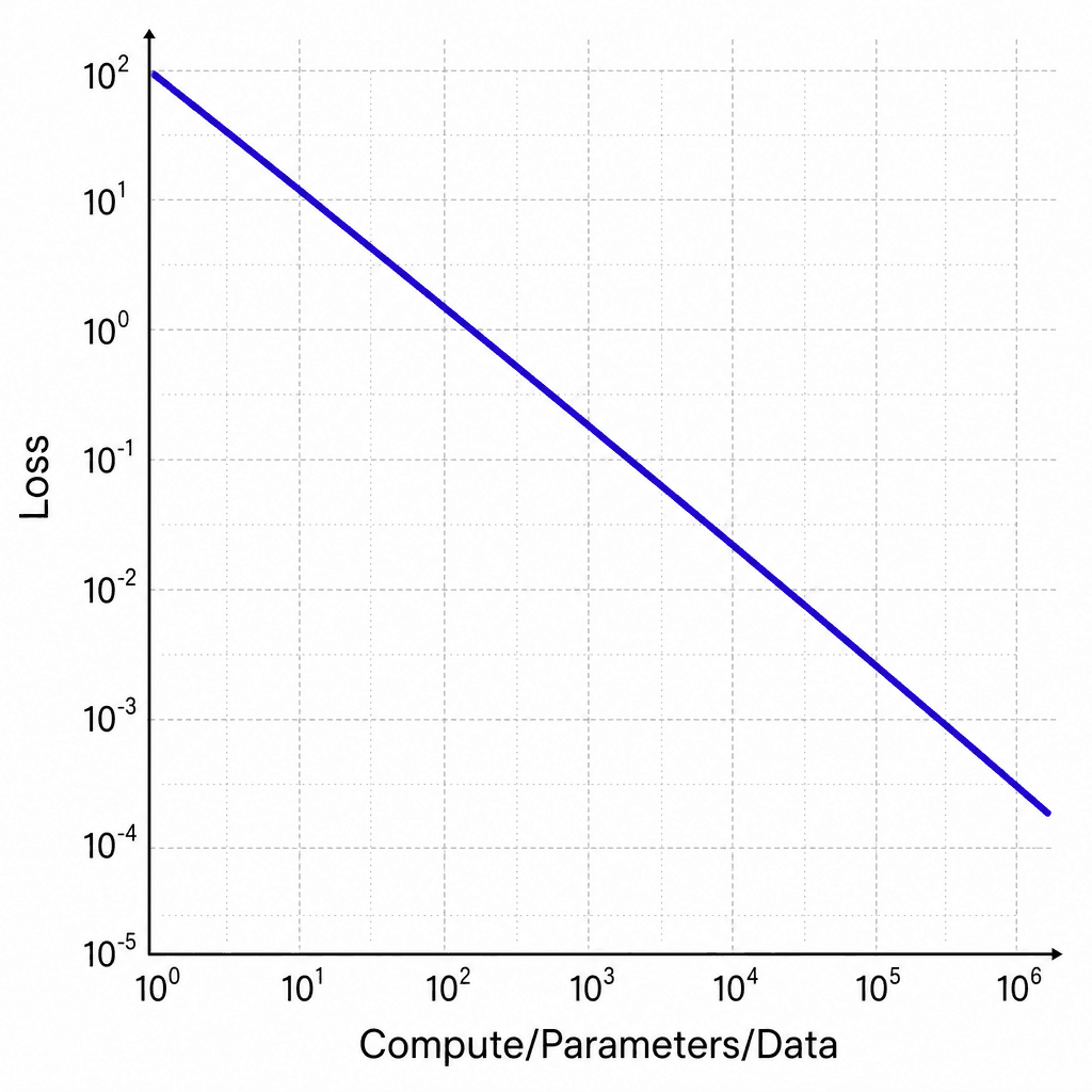
The foundational observation is that loss decreases as a power law with respect to these variables. Mathematically, this is expressed as:

$L(N, D) = A N^{-\alpha} + B D^{-\beta} + E$

Where $L$ is the loss, $A$, $B$, and $E$ are constants, and $\alpha$ and $\beta$ are positive exponents. The key insight here is linearity on a log-log plot. If you double the number of parameters, the loss drops by a predictable factor. If you double the data, the loss drops by another predictable factor. This predictability allows engineers to forecast performance before training begins.

However, this relationship holds only within certain bounds. It assumes that the model is not bottlenecked by other factors, such as optimization algorithms or data quality. Because of the shape of this power law, as models grow larger, each additional parameter yields less marginal improvement than the last, even though the exponent $\alpha$ itself is treated as roughly constant across scales.

The Chinchilla Compute Optimal Strategy

For years, the industry followed a heuristic of maximizing model size while treating data as an afterthought. This led to massive models trained on relatively small datasets, resulting in inefficient use of compute. The Chinchilla paper (DeepMind Paper) overturned this assumption by identifying the "compute optimal" point.

The mechanism behind Chinchilla’s strategy is simple but counterintuitive: if you double the number of parameters, you must also double the number of training tokens to maintain optimality. Previous models like GPT-3 (OpenAI Paper) were significantly undertrained relative to their size. Chinchilla demonstrated that a smaller model trained on more data outperforms a larger model trained on less data, given the same compute budget.

Consider two models, Model A and Model B, with the same total compute budget $C$. Model A has twice the parameters of Model B but half the training data. According to the Chinchilla principle, Model B will achieve lower loss because it has fully utilized the information available in the dataset. Model A, conversely, has memorized its small dataset without generalizing effectively, leading to higher test loss despite its larger capacity.

For engineering managers, this means that "bigger is better" is a flawed metric. The correct metric is "balanced is better." Allocating compute to data preprocessing and curation is often more valuable than simply buying more GPU hours to train a larger architecture.

Overtraining and the Limits of Scaling

While scaling laws provide a clear path for growth, they do not guarantee infinite improvement. When a model is trained on far more tokens than the Chinchilla compute-optimal ratio calls for given its parameter count, it enters the regime of overtraining. Overtraining occurs when additional training tokens keep reducing loss, but at a steeply diminishing rate, so the compute spent no longer buys a proportional improvement in performance.

As models scale, they exhibit "emergent abilities"—capabilities that appear abruptly rather than gradually. However, these abilities are not always beneficial. Overtraining can lead to brittle models that perform well on benchmarks but fail in production environments due to distributional shifts.

Further exploration suggests that there are diminishing returns to increasing model size when the dataset is fixed. The mechanism here is related to the capacity of the model to compress information. Once the model has learned all the patterns present in the data, additional parameters only serve to memorize noise. This is why data quality becomes paramount. A smaller model trained on pristine, diverse data will outperform a larger model trained on noisy, repetitive data.

For engineers, this means that monitoring validation loss is not enough. You must also monitor the gap between training and validation loss. If this gap widens significantly, you are overfitting, and adding more compute or parameters will not help. Instead, you must improve the dataset.

Forecasting Future Performance

Scaling laws are not just retrospective explanations; they are predictive tools. By fitting a power law to current performance data, engineers can forecast the compute required to reach a target loss. This is essential for planning research roadmaps and budgeting for infrastructure.

The process involves collecting data points from existing models (parameters, data size, loss) and performing a linear regression on the log-log scale. The resulting equation allows you to solve for $N$ or $D$ given a target $L$ and a fixed compute budget $C$.

However, forecasting is subject to uncertainty. The exponents $\alpha$ and $\beta$ are not constant across all scales. As models become extremely large, the efficiency of attention mechanisms and the quality of data may introduce non-linearities that deviate from the simple power law. Therefore, forecasts should be treated as estimates with confidence intervals, not guarantees.

Moreover, the forecast assumes that the algorithmic complexity remains constant. Breakthroughs in architecture, such as the shift from dense transformers to mixture-of-experts (MoE) models, can shift the scaling curve entirely. MoE models allow for larger effective parameter counts without proportional increases in compute cost, effectively changing the value of $C$ in the scaling equation.

Common Pitfalls

When applying scaling laws, teams often fall into specific traps that hinder progress. Being aware of these pitfalls is crucial for effective resource management.

1. Ignoring Data Quality for Model Size: Many teams assume that throwing more parameters at a problem will compensate for poor data. In reality, a high-quality, curated dataset will consistently outperform a larger model trained on noisy or uncurated data.
2. Assuming Scaling Laws Are Constant Across Architectures: Scaling exponents vary depending on the model architecture (e.g., dense vs. sparse MoE). Applying scaling laws derived from dense transformers to MoE models without adjustment can lead to significant miscalculations in resource requirements.
3. Overfitting on Synthetic Data: As high-quality human-generated data becomes scarce, teams increasingly turn to synthetic data. However, synthetic data often lacks the diversity and nuance of human text, leading to rapid overfitting where the model memorizes artifacts of the generation process rather than learning generalizable patterns.

Practical Takeaways

To make the most of scaling laws in your engineering workflow, consider these mental models and rules of thumb:

1. Balance Compute Between Parameters and Data: Follow the Chinchilla principle. If you increase model size, proportionally increase data volume. Do not let one side of the equation lag significantly behind the other.
2. Monitor Validation Loss Gap: Keep a close eye on the divergence between training and validation loss. A widening gap is the primary indicator of overfitting and suggests that more compute will not improve generalization.
3. Forecast with Confidence Intervals: When planning for future model capabilities, treat scaling law predictions as ranges rather than precise numbers. Account for potential architectural breakthroughs and data quality improvements that could shift the curve.

FAQ

Q: What is the Chinchilla compute optimal strategy? A: The Chinchilla strategy posits that for a fixed compute budget, model size and dataset size should be scaled equally. Doubling the number of parameters requires doubling the number of training tokens to maintain optimal performance, challenging the previous industry norm of prioritizing model size over data quantity.

Q: How do scaling laws help with forecasting? A: Scaling laws allow engineers to fit a power law curve to existing model performance data. This enables the prediction of the compute resources required to achieve a specific target loss, helping teams plan research roadmaps and infrastructure budgets effectively.

Q: What is overtraining in the context of large language models? A: Overtraining occurs when a model is trained on more tokens than the Chinchilla compute-optimal ratio calls for given its parameter count. Additional tokens continue to lower loss, but at a steeply diminishing rate, so the compute spent yields a much smaller return than a compute-optimal allocation would.