pgvector at 100 Million Vectors: Lessons Learned

Scaling a vector database in Postgres is often assumed to be a matter of throwing more RAM at the server. When you hit 100 million vectors, however, the problem shifts from storage capacity to memory locality, index construction stability, and concurrency control. If you treat pgvector like a standard B-tree index, you will likely encounter Out-Of-Memory (OOM) errors during creation or unacceptably high latency during query time.

Here are the specific mechanisms that break at scale and how to tune them.

The HNSW Memory Topology

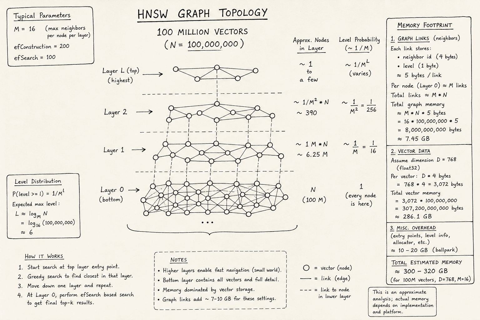
HNSW (Hierarchical Navigable Small World) indexes are not static structures; they are layered graphs. At 100 million vectors, the sheer number of edges creates a memory footprint that exceeds typical maintenance_work_mem settings, causing index creation to fail even if you have terabytes of disk space.

The core mechanism of HNSW involves two key parameters: M (the maximum number of connections per node in each layer) and efConstruction (the size of the dynamic candidate list during index building). During index tuning, these parameters dictate the balance between build time, memory usage, and search quality.

At scale, the memory required for an HNSW index is approximately:

$\text{Memory} \approx N \times M \times \text{layer\_height} \times \text{vector\_size}$

Where $N$ is the number of vectors. For 100 million vectors with 768-dimensional floats, even a modest M=16 can require several gigabytes of RAM just for the index structure itself, excluding the base table data. Note that this is a rough heuristic; actual memory usage depends heavily on the random graph generation process and the variable number of edges per layer.

Lesson 1: Tune maintenance_work_mem aggressively.

When creating the index, Postgres uses maintenance_work_mem to allocate temporary structures for sorting and merging graph layers. If this value is too low, the index builder falls back to disk-based sorting, which is exponentially slower and often fails for large graphs due to file descriptor limits or fragmentation.

-- During index creation, set high memory allowance
SET maintenance_work_mem = '8GB';
CREATE INDEX idx_vectors_hnsw ON vectors USING hnsw (embedding vector_cosine_ops);

Do not leave this at the default 64MB. For 100M vectors, 4GB–8GB is often the minimum stable threshold for maintenance_work_mem to keep the construction process in-memory.

Partitioning for Write Concurrency

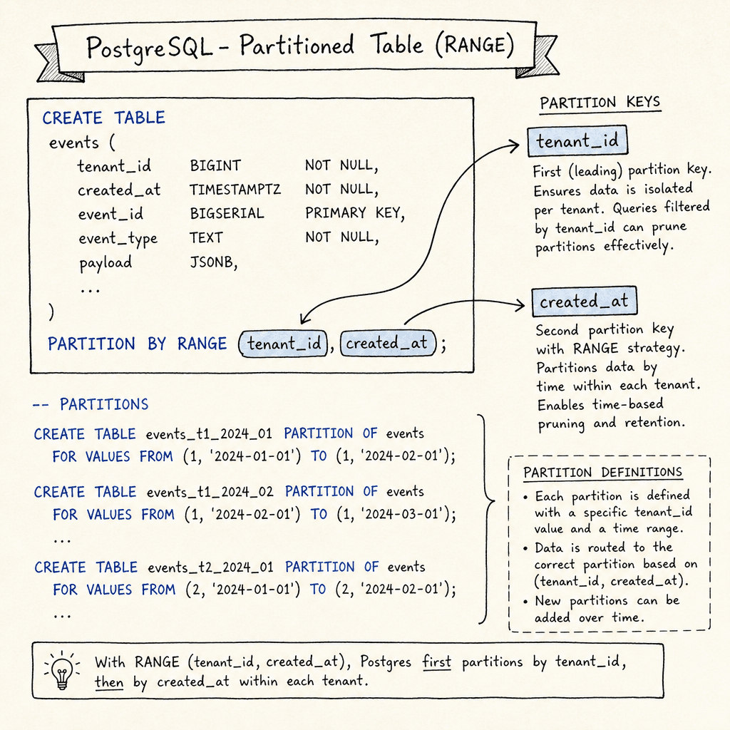
A common misconception is that partitioning pgvector is primarily for data lifecycle management (e.g., dropping old data). While useful, the primary engineering benefit at 100M vectors is write concurrency.

HNSW indexes are mutable. In pgvector, updates typically lock the heap tuple and trigger a rebuild of the index entry for that specific vector. However, at scale, the cost of these individual rebuilds and the resulting heap lock contention can become significant bottlenecks. By applying partitioning strategies, such as range partitioning by created_at or tenant_id, you distribute the index across multiple physical segments. This reduces the lock contention because writes to partition A do not block reads or writes to partition B.

Lesson 2: Use range partitioning to isolate index writes.

CREATE TABLE vectors (
    id bigserial PRIMARY KEY,
    tenant_id int NOT NULL,
    embedding vector(768),
    created_at timestamptz DEFAULT now()
) PARTITION BY RANGE (created_at);
 
CREATE TABLE vectors_2023_q4 PARTITION OF vectors
    FOR VALUES FROM ('2023-10-01') TO ('2024-01-01');
 
CREATE TABLE vectors_2024_q1 PARTITION OF vectors
    FOR VALUES FROM ('2024-01-01') TO ('2024-04-01');

Each partition gets its own HNSW index. This means that a burst of writes to the current quarter’s partition only locks that specific index. The historical partitions remain read-only or append-only, allowing for faster VACUUM operations and reduced bloat.

Query Tuning: Latency vs. Recall

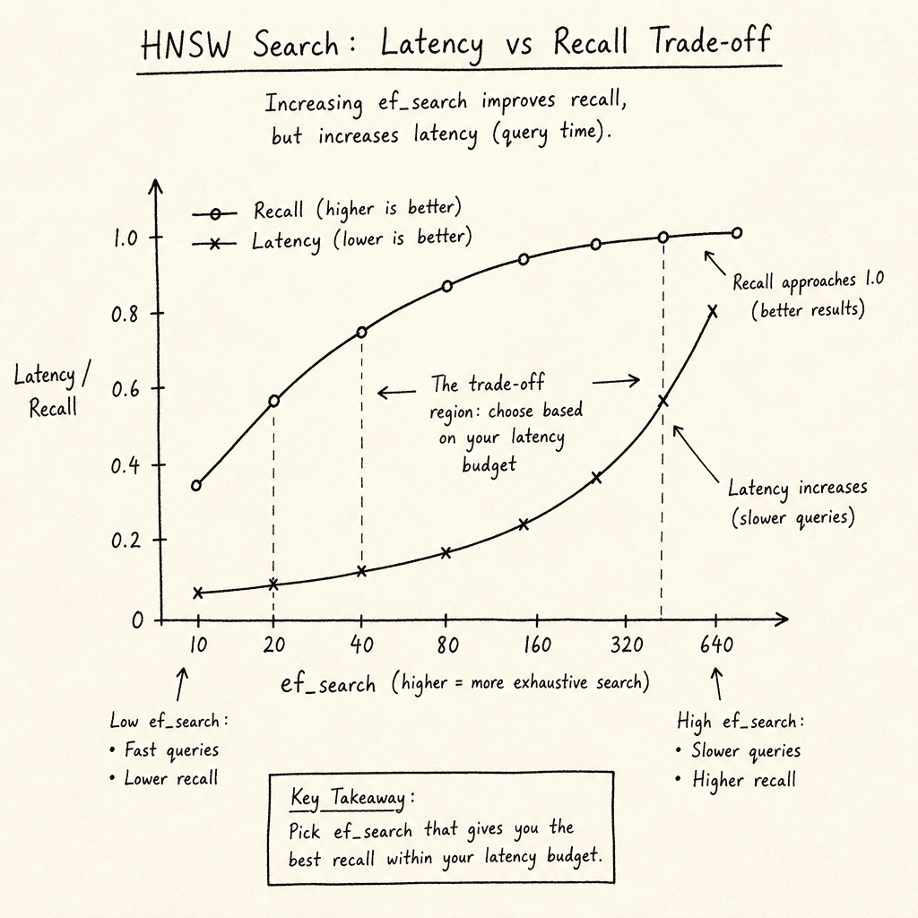
At 100 million vectors, the default hnsw.ef_search value (usually 40) is often insufficient for high-recall requirements but excessive for low-latency needs. The ef_search parameter controls the size of the dynamic candidate list during query traversal.

Mechanistically, HNSW performs a greedy search down the layers. A higher ef_search means the algorithm explores more nodes before committing to a path, increasing accuracy (recall) but also CPU time and I/O. As you focus on scaling your dataset, profiling this parameter becomes critical to balancing throughput against accuracy.

Lesson 3: Profile hnsw.ef_search per workload.

Do not set hnsw.ef_search globally. Instead, use session-level or connection-level configuration based on the application’s latency budget.

-- For high-recall admin queries
SET hnsw.ef_search = 200;
SELECT * FROM vectors ORDER BY embedding <-> query_vector LIMIT 10;
 
-- For low-latency user-facing queries
SET hnsw.ef_search = 40;
SELECT * FROM vectors ORDER BY embedding <-> query_vector LIMIT 10;

Benchmark your specific data distribution. Some datasets have "clumpy" vector spaces where recall stabilizes at ef_search=100, while others require ef_search=500+ to avoid missing relevant neighbors. Always measure recall against a brute-force KNN result to quantify the trade-off.

Vacuuming and Index Bloat

In pgvector, each UPDATE to an embedding is implemented internally as a delete followed by an insert, leaving the old graph node behind as a dead tuple. Since pgvector 0.6.0, VACUUM can reclaim these dead tuples, but it does not rebalance or compact the underlying graph structure. Consequently, VACUUM alone is often not sufficient to fully restore search performance after heavy update volume.

If you frequently update embeddings, the index grows larger than necessary, slowing down search. For partitioned tables, regular maintenance is essential. In Postgres 15+, VACUUM is more efficient for heap cleanup, but for HNSW, consider using REINDEX if you notice significant performance degradation over time, especially after bulk updates. This index tuning step is crucial for scaling operations where write-heavy workloads create significant graph fragmentation.

-- Reindex a specific partition
REINDEX INDEX vectors_2024_q1_hnsw_idx;

Conclusion

Scaling pgvector to 100 million vectors is achievable without external vector databases, but it requires respecting the memory and locking mechanics of HNSW. Key takeaways for scaling your vector workload include:

1. Memory: Set maintenance_work_mem high during index creation.
2. Concurrency: Use range partitioning to isolate write locks.
3. Latency: Tune hnsw_ef_search per query type, not globally.
4. Maintenance: Monitor index size and reindex periodically after bulk updates.

These adjustments transform pgvector from a novelty into a production-grade vector store capable of handling enterprise-scale workloads.