Metadata Filtering at Scale: Vector Search

The Hidden Cost of Metadata Filtering in Vector Search

Vector search is often marketed as a drop-in replacement for traditional keyword search. This is misleading. While vector search excels at semantic similarity, it is structurally blind to discrete metadata attributes like tenant_id, created_at, or status. When you add metadata filtering, you are not just adding a condition; you are introducing a fundamental tension between recall (finding all relevant items) and latency (doing it quickly).

This is Part 4 of the Retrieval Engineering series.

For backend developers building multi-tenant systems, this tension is the primary bottleneck. If you filter naively, you pay an O(N) penalty for every query. If you index poorly, you waste storage and memory. This post explains the mechanism-level tradeoffs of maintaining selectivity at scale.

The Selectivity Problem

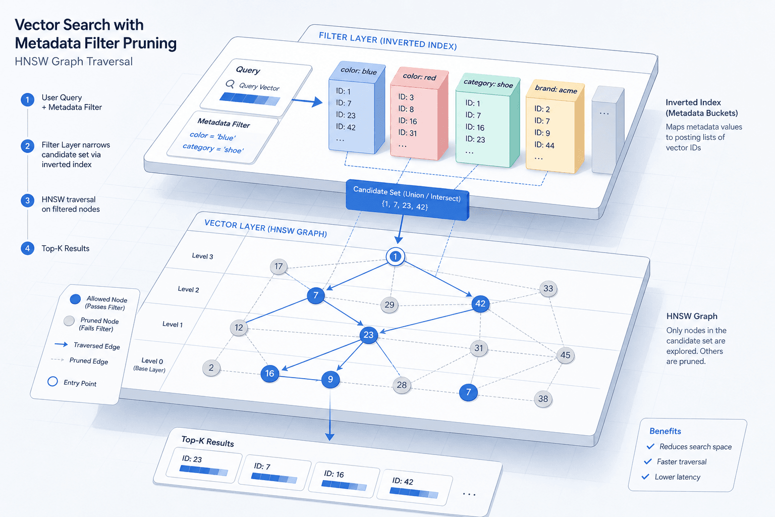
To understand why filtering is hard, we must look at how vector indices work. Most production systems use Hierarchical Navigable Small World (HNSW) graphs. These graphs allow approximate nearest neighbor (ANN) search in logarithmic time by navigating a hierarchy of sparse graphs.

The problem arises when you apply a metadata filter after the vector search completes.

Consider a database with 10 million vectors. You query for a semantic match, but you only want results from tenant_id: "acme-corp". If your index does not support efficient pre-filtering, the system must:

1. Retrieve the top K candidates from the HNSW graph (e.g., 100 results).
2. Fetch the full metadata payload for those 100 vectors.
3. Filter out results that don't match tenant_id.

This seems fine until selectivity drops. Suppose tenant_id is not unique, or you are querying a common tag. If the filter only reduces the candidate set from 10 million to 5 million, the HNSW traversal becomes inefficient because it has to traverse a much larger portion of the graph to find the true nearest neighbors within that filtered subset.

In the worst case, naive filtering forces a full scan or a massive reduction in recall, as the algorithm stops searching early to meet latency constraints, missing valid matches that lie outside the initial high-probability zone.

Payload Indexing: The Mechanism

The solution is not to filter after the fact, but to integrate metadata into the search structure. This is achieved through payload indexing.

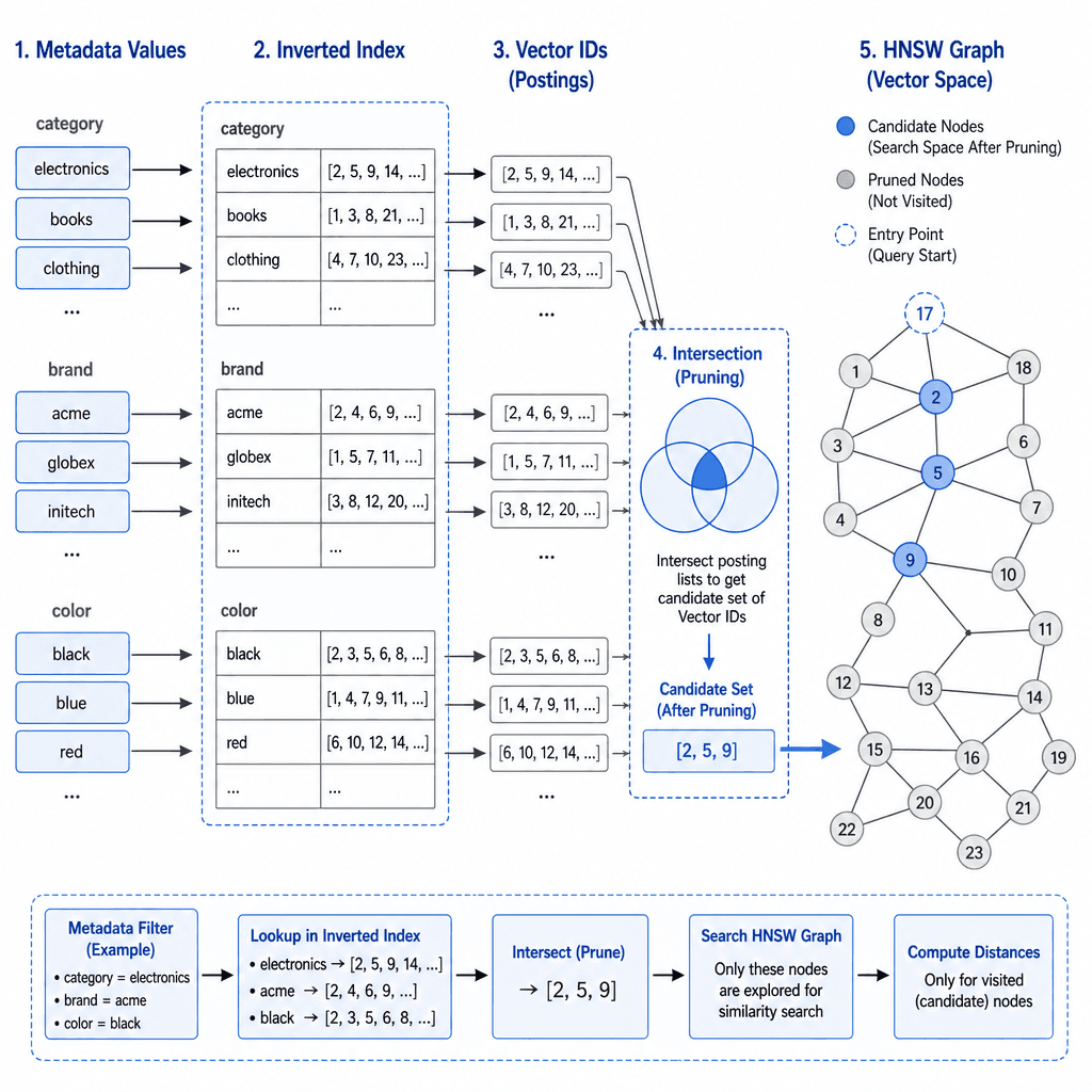
Payload indexing involves creating an auxiliary data structure (typically an inverted index or a bitmap index) that maps metadata values to vector IDs. When a query arrives, the system:

1. Looks up the vector IDs associated with the filter criteria (e.g., all IDs where tenant_id = "acme-corp").
2. Intersects this set with the HNSW search results or restricts the HNSW traversal to only those IDs.

How It Works Under the Hood

Most modern vector databases (Pinecone, OpenSearch, Milvus) implement this by storing metadata alongside the vector embeddings in the same shard or node. However, the efficiency depends on the index type:

• Inverted Index: Maps metadata values to lists of vector IDs. Efficient for high-cardinality filters but consumes more memory.
• Bitmap Index: Uses bitmaps to represent the presence of metadata values. Highly efficient for low-cardinality filters (e.g., boolean flags) but can become sparse and inefficient for high-cardinality data.

For example, in OpenSearch, you can define a knn field alongside a filter field. The query engine uses the filter to prune the search space before invoking the HNSW algorithm.

GET /products/_search
{
  "size": 10,
  "query": {
    "knn": {
      "embedding": {
        "vector": [0.1, 0.2, ...],
        "k": 10,
        "filter": {
          "bool": {
            "filter": [
              { "term": { "tenant_id": "acme-corp" } },
              { "range": { "price": { "gte": 10 } } }
            ]
          }
        }
      }
    }
  }
}

Here, the filter clause is processed first, reducing the candidate set before the expensive vector distance calculations occur. This is the key mechanism for maintaining low latency.

Multi-Tenant Isolation Strategies

In multi-tenant architectures, metadata filtering is often used for isolation. Each tenant's data must be strictly separated. There are two primary approaches:

1. Logical Isolation (Filter-Based)

All tenants share the same vector index, but queries include a tenant_id filter. This is simple to implement but suffers from the selectivity problem described above if the index is large and tenants have varying data volumes.

Pros: Simple setup, shared infrastructure. Cons: Cross-tenant noise, potential for slower queries if filters are not selective, complex to manage index scaling.

2. Physical Isolation (Namespace/Shard-Based)

Each tenant gets their own index or shard. Queries are routed directly to the relevant tenant's index. This is the gold standard for strict isolation and performance.

Pros: No cross-tenant leakage, independent scaling, no filter overhead. Cons: Complex operational overhead, higher storage costs due to index duplication, harder to perform cross-tenant analytics.

For most SaaS applications, a hybrid approach works best: use physical isolation for large enterprise tenants and logical isolation for smaller tenants, grouped into logical "shards."

Selectivity Optimization Techniques

Beyond payload indexing, several techniques can optimize selectivity:

Pre-Computed Metadata Filters

Instead of storing raw metadata and filtering at query time, pre-compute common filter combinations. For example, if you frequently query status: "active" AND category: "electronics", create a secondary index that maps this combination to vector IDs. This reduces the search space dramatically.

Hybrid Search

Combine vector search with traditional keyword search. Use the keyword search to filter down to a small, relevant subset of documents, then apply vector search within that subset. This leverages the precision of BM25 for metadata filtering and the recall of vectors for semantic matching.

Hierarchical Filtering

Implement a two-tier filtering system. First, filter on high-selectivity metadata (e.g., tenant_id, user_id) to reduce the candidate set to thousands. Then, apply lower-selectivity filters (e.g., category, tags) within that smaller set. This minimizes the number of vectors the HNSW graph needs to traverse.

Conclusion

Metadata filtering in vector search is not an afterthought; it is a core architectural decision. Naive filtering leads to poor latency and recall. By integrating payload indexes, choosing the right isolation strategy, and optimizing selectivity, you can build vector search systems that are both fast and scalable. The key is to move filtering from the post-processing stage to the index traversal stage, ensuring that the HNSW graph only explores relevant regions of the vector space.

Common Pitfalls

1. Ignoring Selectivity: Applying filters that reduce the candidate set by only a small percentage often costs more in latency than the filter saves, especially if the index is large. Always measure the selectivity of your filters.
2. Over-Indexing: Creating payload indexes for every metadata field increases storage overhead and write latency. Only index fields that are frequently used in filters or have high cardinality where bitmap indexes would be inefficient.
3. Post-Processing Bias: Relying on post-hoc filtering (retrieving K results, then filtering) introduces bias. If the filter excludes many of the top K results, the system may return fewer than K results or require a much larger K, increasing latency unpredictably.

Practical Takeaways

• Pre-filter, don't post-filter: Integrate metadata into the HNSW traversal using payload indexes to prune the search space early.
• Choose the right index type: Use inverted indexes for high-cardinality filters and bitmap indexes for low-cardinality filters to balance memory and speed.
• Optimize for selectivity: Structure queries to filter on high-selectivity attributes first, reducing the candidate set before expensive vector calculations.
• Isolate strategically: Use physical isolation for strict multi-tenant security and logical isolation for shared, less sensitive data to balance complexity and performance.

FAQ

Q: Does payload indexing increase storage costs? A: Yes, payload indexes (like inverted indexes) require additional storage to map metadata values to vector IDs. However, this is often outweighed by the performance gains in query latency.

Q: Can I use metadata filtering with any vector database? A: Most modern vector databases support some form of metadata filtering, but the implementation details (e.g., HNSW integration, index types) vary. Check your specific database's documentation for supported filter types.

Q: What is the difference between logical and physical isolation? A: Logical isolation uses filters within a shared index, while physical isolation uses separate indexes or shards for each tenant. Physical isolation offers better performance and security but is harder to manage.

Q: How do I handle high-cardinality metadata like user IDs? A: High-cardinality fields are best handled with inverted indexes or by treating them as unique identifiers in a physical isolation model, rather than trying to use bitmap indexes which become inefficient with many unique values.