ANN Indexes: HNSW, IVF, and DiskANN Compared

Vector search faces a fundamental bottleneck: the "curse of dimensionality." As vector dimensions increase, the distance between points becomes uniform, rendering brute-force linear search ($O(N)$) computationally infeasible for large datasets. To solve this, Approximate Nearest Neighbor (ANN) algorithms introduce approximations that sacrifice exact precision for significant gains in speed and memory efficiency. Three dominant algorithms—HNSW, IVF, and DiskANN—employ distinct mechanisms to navigate high-dimensional space. Understanding these mechanisms is critical for backend engineers selecting indexes for production systems.

Many backend teams struggle with ANN selection because they treat it as a simple library configuration rather than a hardware-aware architectural decision. In practice, the gap between benchmarked recall and production performance often stems from ignoring memory overhead or underestimating the tuning complexity required for disk-based indexes. This article is Part 2 of the Retrieval Engineering series.

HNSW: The Layered Graph Mechanism

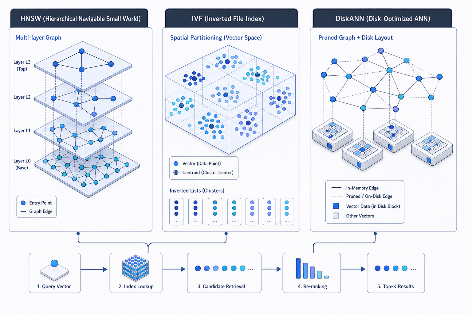
Hierarchical Navigable Small World (HNSW) indexes vectors using a multi-layered graph structure. The core mechanism relies on the "small world" property, where most nodes are reachable via short paths despite the graph's large size.

HNSW builds this structure by inserting vectors into a hierarchy of graphs. The bottom layer contains all vectors, while upper layers contain progressively fewer vectors, acting as "express lanes." When inserting a new vector, the algorithm determines its optimal position in the topmost layer, then descends layer by layer, finding the nearest neighbors in each layer to form edges. This randomised insertion strategy ensures the graph maintains a logarithmic diameter, a property detailed in the original HNSW paper by Malkov & Yashunin.

Search begins at the top layer with a single entry point. The algorithm finds the nearest neighbor in that layer, then moves down to the next layer, using the previous layer's result as the starting point. This "greedy search" skips vast portions of the dataset that are far from the query. The search is controlled by two key parameters: M (the maximum number of connections per node) and efConstruction (the search depth during index building). Higher M values improve recall but increase memory usage and build time; higher efConstruction improves index quality but slows construction.

During query time, HNSW uses a parameter efSearch to control the search breadth. A higher efSearch explores more nodes, increasing recall at the cost of latency. Note that efSearch is often exposed as ef in libraries like Milvus to prevent practitioner confusion. Because HNSW operates entirely in RAM, query latency is typically sub-millisecond for millions of vectors, making it ideal for low-latency applications like recommendation engines. However, the graph structure requires storing $O(N \cdot M)$ edges, leading to significant memory overhead.

IVF: Spatial Partitioning and Quantization

Inverted File (IVF) indexes take a different approach: spatial partitioning. Instead of a graph, IVF divides the vector space into clusters using k-means clustering. Each cluster is represented by a centroid. The index stores an inverted list for each centroid, containing the vectors assigned to that cluster.

Search proceeds in two stages. First, the algorithm identifies the $K$ nearest centroids to the query vector. This step reduces the search space from $N$ vectors to only those within the selected clusters. Second, the algorithm computes distances only for vectors within these clusters. This mechanism drastically reduces the number of distance calculations compared to brute force, a concept foundational to libraries like FAISS and Milvus.

To further optimize memory, IVF is often combined with Product Quantization (PQ). PQ compresses each vector into a short code by dividing the vector into subspaces and mapping each subspace to the nearest centroid in a small codebook. This reduces the storage footprint by orders of magnitude, allowing more vectors to fit in RAM. However, PQ introduces approximation error because the compressed code is an estimate of the original vector.

The latency of IVF depends on the number of clusters ($nlist$) and the number of probes ($nprobe$). Increasing nprobe improves recall by searching more clusters but increases latency. Unlike HNSW, IVF does not guarantee logarithmic search time; performance can degrade if the query falls near cluster boundaries, requiring more probes. IVF is highly effective for large datasets where RAM is constrained, as the compressed codes allow higher density storage than HNSW's graph edges.

DiskANN: Bridging RAM and Disk

DiskANN addresses the limitation of RAM-bound indexes like HNSW and IVF. When datasets exceed available memory, traditional indexes require paging or swapping, causing catastrophic latency spikes. DiskANN uses a compressed graph structure optimized for disk I/O.

DiskANN builds a pruned graph similar to HNSW but removes edges that are rarely used in search paths, reducing the graph size. It then partitions this graph into pages that fit into disk blocks. During search, DiskANN uses a small candidate list of nodes to guide the search into the correct disk pages. This mechanism minimizes disk seeks by ensuring that each page load yields useful candidates. This architecture was detailed in the DiskANN paper by Subramanya et al.

DiskANN also employs aggressive quantization, including binary and scalar quantization, to reduce the size of each node's vector representation. This allows the entire index to reside on disk while maintaining high recall. Note that specific quantization methods and their efficacy vary by implementation version (e.g., Vamana vs. later iterations), so engineers should verify the specific compression techniques supported by their chosen library. The trade-off is latency: disk reads are slower than RAM accesses, so query times are typically in the tens of milliseconds rather than sub-millisecond. However, DiskANN can handle billions of vectors on commodity hardware, where HNSW would require terabytes of RAM.

The key innovation of DiskANN is its ability to balance recall and latency by tuning the number of nodes searched per page. By limiting the search depth within each page, it avoids unnecessary disk reads while maintaining high recall. This makes DiskANN suitable for large-scale search applications where storage cost is a primary concern, such as web-scale image or text retrieval.

Comparative Analysis: Trade-offs in Production

Selecting an index requires balancing recall, latency, and resource constraints. HNSW offers the lowest latency and stable recall, making it ideal for real-time applications with moderate dataset sizes (<10 million vectors) and sufficient RAM. Its memory overhead is linear with the number of edges, so it becomes expensive at scale.

IVF is the go-to choice for large datasets where RAM is limited. It offers a good balance between memory efficiency and query speed, especially when combined with PQ. However, recall can be less stable than HNSW, particularly for queries near cluster boundaries. IVF is best suited for batch processing or applications where slight latency variations are acceptable.

DiskANN is designed for massive datasets (>100 million vectors) that exceed RAM capacity. It provides high recall at the cost of higher latency due to disk I/O. It is optimal for scenarios where storage cost is critical, and sub-second latency is acceptable. DiskANN's complexity in tuning and deployment makes it less suitable for small-scale applications.

Quantization plays a crucial role in all three indexes. HNSW can use PQ to reduce memory usage, but this may impact recall. IVF relies on PQ for efficiency, and DiskANN uses aggressive quantization to fit the graph on disk. Engineers must validate recall metrics after applying quantization, as aggressive compression can degrade search quality.

In summary, HNSW prioritizes speed, IVF prioritizes memory efficiency, and DiskANN prioritizes scalability. The choice depends on the specific constraints of the production environment, including dataset size, available hardware, and latency requirements.

Conclusion

Choosing the right ANN index is not about finding the "best" algorithm, but about matching the algorithm's mechanism to your system's constraints. HNSW wins on latency, IVF on memory efficiency, and DiskANN on scale. By understanding the underlying mechanics of graph navigation, spatial partitioning, and disk paging, you can make informed decisions that balance performance, cost, and complexity in your vector search infrastructure.

Actionable Next Steps

Audit your current index configuration against these trade-offs. Start by profiling your recall requirements before selecting HNSW or IVF. If you are managing datasets over 100 million vectors, evaluate DiskANN's disk I/O characteristics against your hardware's read speeds to ensure latency targets are met.

Common Pitfalls

1. Ignoring HNSW Memory Overhead: Assuming HNSW scales linearly without accounting for edge storage. At 100M+ vectors, the memory footprint can become prohibitive if M is not carefully tuned.
2. Underestimating DiskANN Tuning Complexity: Treating DiskANN as a drop-in replacement for in-memory indexes. It requires careful tuning of page sizes and search depths to avoid excessive disk seeks, which can lead to unpredictable latency spikes.
3. Blindly Applying PQ: Using Product Quantization without validating recall loss. Aggressive quantization can significantly degrade search quality, especially for datasets with high variance in vector norms.

Practical Takeaways

• Latency Priority: Choose HNSW for sub-millisecond responses in RAM-constrained environments.
• Memory Efficiency: Choose IVF with PQ for large datasets where RAM is limited but latency can tolerate slight variations.
• Scale Priority: Choose DiskANN for billion-vector indexes where storage cost is the primary constraint and sub-second latency is acceptable.

FAQ

Can I use HNSW for billions of vectors? Technically yes, but it is often impractical due to memory overhead. HNSW stores $O(N \cdot M)$ edges, which can require terabytes of RAM for billions of vectors. For such scales, DiskANN or IVF is more cost-effective.

How does PQ affect recall? Product Quantization introduces approximation error by compressing vectors into codes. The impact on recall depends on the number of subspaces and the codebook size. Generally, higher compression leads to lower recall. Always benchmark recall after applying PQ.

Is DiskANN faster than IVF? DiskANN is generally slower in terms of query latency due to disk I/O, but it allows for much larger datasets to be searched within the same hardware constraints. IVF is faster if the dataset fits in RAM, but DiskANN scales better in terms of storage efficiency.

Do I need to retrain my model if I change indexes? No, the ANN index is independent of the embedding model. However, changing indexes may require re-tuning parameters (like M, efSearch, or nprobe) to achieve similar recall levels.