Why Quantization Works: Precision, Range, and Outliers

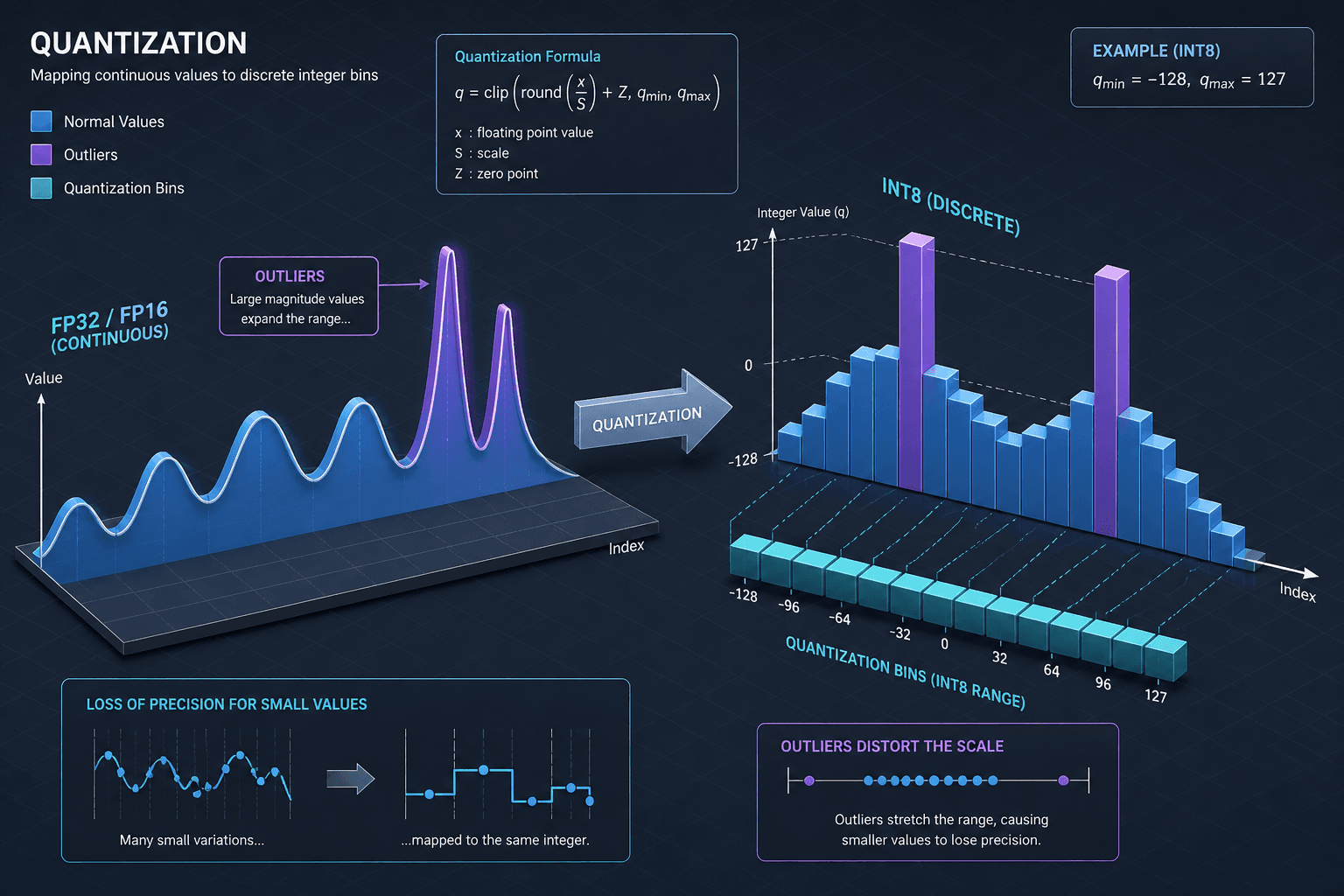
Quantization is a lossy compression scheme that maps continuous floating-point numbers to discrete integers. For ML engineers, understanding why it fails is critical. Failure modes are mathematical consequences of dynamic range limitations and activation value distributions. This article dissects fp16 and int8 mechanics, focusing on precision loss and outlier disruption.

The Mechanics of fp16: Trading Range for Precision

Half-precision floating point (fp16 or float16) is a 16-bit format defined by the IEEE 754-2019 standard¹. It is not a "compressed" version of fp32; it is a distinct format with different structural constraints.

An fp16 value consists of:

• 1 sign bit
• 5 exponent bits
• 10 fraction (mantissa) bits

Compare this to fp32 (single precision), which has 8 exponent bits and 23 fraction bits. The mechanism here is a direct trade-off. By reducing the exponent from 8 to 5 bits, fp16 reduces its maximum representable number from approximately $3.4 \times 10^{38}$ to $6.55 \times 10^4$. More critically, reducing the mantissa from 23 to 10 bits drastically reduces precision. In fp32, the gap between consecutive representable numbers (machine epsilon) near 1.0 is $2^{-23} \approx 1.19 \times 10^{-7}$. In fp16, it is $2^{-10} \approx 9.77 \times 10^{-4}$.

This means that fp16 cannot distinguish between numbers that are very close together. When performing matrix multiplications in deep learning, these small rounding errors accumulate. However, fp16 often works well because neural network weights and activations are not uniformly distributed; they cluster around zero, and the relative error introduced by reduced precision often falls within the model's tolerance for noise.

Modern hardware often pairs fp16 with bf16 (bfloat16) to mitigate these limitations. bf16 retains the full 8-bit exponent range of fp32 but truncates the mantissa to 7 bits. This design preserves the dynamic range, effectively eliminating the overflow issues that plague fp16 during training or inference in modern Transformer architectures, while still offering significant memory bandwidth savings over fp32.

The choice between fp16 and bf16 often comes down to the specific model sensitivity. For instance, in BERT-based models, fp16 can sometimes lead to instability due to gradient underflow, whereas bf16 maintains stability. Conversely, for simpler models like ResNet-50, fp16 often suffices without significant accuracy degradation, demonstrating that the success of half-precision is highly data-dependent.

The Int8 Mapping Problem: Uniform Bins

int8 quantization is more aggressive. It maps floating-point values to an 8-bit signed integer range of $[-128, 127]$. The most common method is linear affine quantization. The mechanism involves two parameters: a scale factor ($s$) and a zero-point ($z$).

The mapping formula is: $x_{int8} = \text{round}\left(\frac{x_{fp32}}{s}\right) + z$

Conversely, to dequantize: $x_{fp32} = s \times (x_{int8} - z)$

Here, $s$ determines the step size between adjacent integers. If $s = 0.01$, then each increment in int8 represents a 0.01 change in the original float. The zero-point $z$ ensures that the float value 0.0 maps exactly to the integer 0 (or the nearest representable integer).

The critical insight is that this mapping creates uniform bins. The distance between the value represented by integer 10 and integer 11 is always $s$. This works well if the data is uniformly distributed. However, neural network activations are rarely uniform. They often follow a heavy-tailed distribution, meaning most values are small, but a few are extremely large.

The Outlier Crisis

Outliers are the primary enemy of int8 quantization. An outlier is a value that is significantly larger than the majority of the data in a tensor.

Consider a layer in a transformer model where most activation values lie between $-0.5$ and $0.5$. However, due to a specific input pattern or attention head behavior, one value spikes to $10.0$.

If we use per-tensor quantization (a single scale factor for the entire tensor), the scale $s$ must be large enough to accommodate the outlier. If the range is $[-10.0, 10.0]$, the scale might be $0.078$ ($20 / 255$).

Now, look at the small values. A value of $0.1$ becomes: $\text{round}(0.1 / 0.078) + z \approx \text{round}(1.28) + z \approx 1 + z$

A value of $0.05$ becomes: $\text{round}(0.05 / 0.078) + z \approx \text{round}(0.64) + z \approx 1 + z$

Both $0.1$ and $0.05$ map to the same integer. The model loses the distinction between them. This is precision collapse. The outlier forces the entire tensor to have a coarse resolution, destroying the fine-grained information contained in the majority of the activations. This is why naive per-tensor quantization often fails in modern Transformer architectures.

Handling Outliers: Per-Channel Quantization

The solution to the outlier crisis is per-channel quantization. Instead of a single scale factor for the entire tensor, we compute a separate scale factor for each output channel (or input channel, depending on the operation).

In a convolutional layer or a fully connected layer, the output is a sum of products along the input channels. Each output neuron aggregates information from all input channels. If one input channel has large outliers, it will dominate the sum for that specific output neuron.

By assigning a unique scale factor $s_i$ to each output channel $i$, we isolate the outliers. The scale $s_i$ is determined by the maximum absolute value in that specific channel's weight or activation tensor. This allows channels with small values to have a small scale (high precision) and channels with large outliers to have a large scale (low precision, but covering the range).

Mechanism:

1. Calculate per-channel max: For each channel $i$, find $M_i = \max(|W_i|)$.
2. Compute per-channel scale: $s_i = M_i / 127$.
3. Quantize: $W_{int8}[i] = \text{round}(W_{fp32}[i] / s_i)$.

Note that "per-channel" typically refers to per-output-channel for weights in linear/conv layers, but can be per-input-channel for activations depending on the specific operator implementation. Always verify the axis of quantization for your specific backend.

This ensures that the quantization error is normalized relative to the magnitude of the values in each channel. The outlier in channel 5 does not force channel 1 to have a coarse scale.

Conclusion

Quantization works because neural networks are robust to noise. However, it is not a universal fix. The choice between fp16 and int8 depends on the hardware support and the acceptable trade-off between range and precision. The choice between per-tensor and per-channel quantization depends on the presence of outliers.

For ML engineers, the key takeaway is that quantization is a data-dependent process. You cannot apply a single scale factor to a tensor with heavy-tailed distributions without losing significant precision. Always inspect the distribution of your activations. If you see outliers, use per-channel quantization. If you see a tight cluster, per-tensor might suffice. Understanding the mechanism of mapping allows you to debug quantization errors rather than guessing.

In the next part of this series, we will explore how to implement these concepts in PyTorch and TensorFlow, including the practical steps of calibration and verification.

Common Pitfalls

1. Ignoring Calibration Data Distribution: Using a calibration set that does not represent the inference distribution can lead to incorrect scale factors. If your training data is balanced but your inference data is skewed, quantization performance will degrade.
2. Using Per-Tensor for Heavy-Tailed Data: As discussed, per-tensor quantization fails when outliers are present. Applying it to Transformer attention outputs without checking for outliers is a common source of accuracy loss.
3. Neglecting Mixed Precision: Not all layers benefit from int8. Some sensitive layers, such as those near the output or in specific attention mechanisms, may require fp16 or fp32 to maintain accuracy. Blindly quantizing the entire model can yield diminishing returns.

Footnotes

1. IEEE Computer Society. (2019). IEEE Standard for Floating-Point Arithmetic. IEEE Std 754-2019. https://ieeexplore.ieee.org/document/8766229 ↩