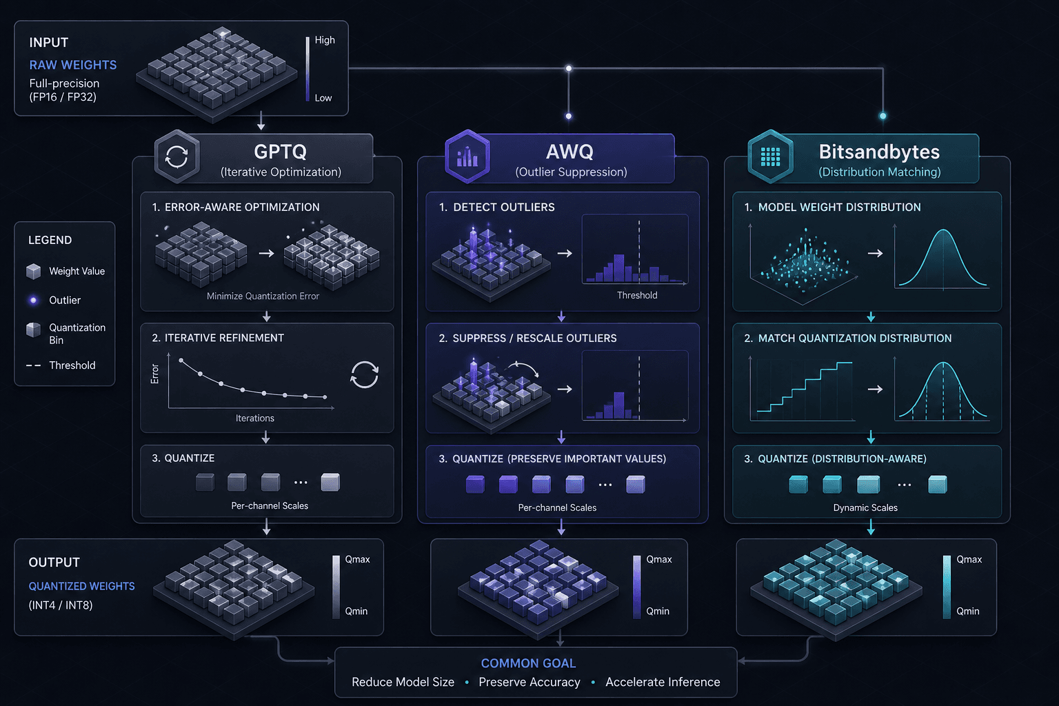
GPTQ vs AWQ vs Bitsandbytes: A Practical Comparison

Quantization is the process of reducing the precision of a model’s parameters to save memory and accelerate inference. For Large Language Models (LLMs), this is not merely a storage optimization; it is a fundamental architectural constraint. The core challenge is that LLM weights follow a heavy-tailed distribution. A small number of "outlier" weights have massive magnitudes, while the majority cluster near zero. Naive uniform quantization fails because these outliers dominate the error budget, causing catastrophic accuracy drops.

Part 3 of the Quantization in Practice series.

To mitigate this, three dominant approaches have emerged: GPTQ, AWQ, and Bitsandbytes (BnB). Each solves the outlier problem differently, leading to distinct trade-offs in calibration complexity, inference speed, and final perplexity.

The Mechanism of Quantization Error

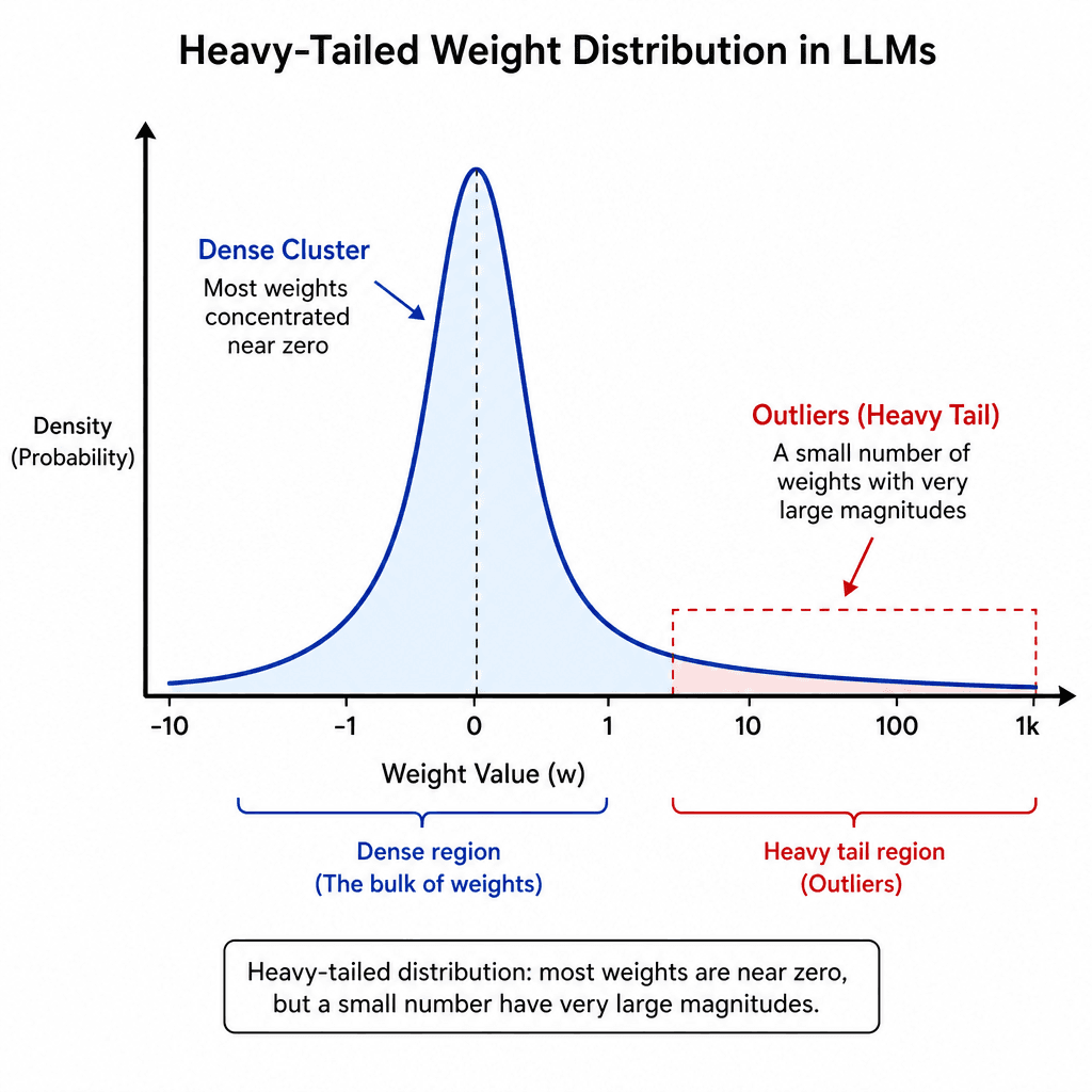
Before comparing tools, we must understand the error source. When we map a continuous float32 weight $w$ to a discrete integer $q$, we introduce quantization noise $\epsilon = w - \hat{w}$. In matrix multiplication $y = Wx$, this noise propagates. If the distribution of $W$ is Gaussian-like, uniform quantization (used in standard INT8) is efficient. However, LLM weights often exhibit "heavy tails."

If we use uniform quantization, the bins must be wide enough to cover the outliers. This results in high quantization error for the dense cluster of small weights. Conversely, if we narrow the bins to fit the dense cluster, the outliers are clipped or severely distorted. The solution requires either:

1. Outlier Suppression: Reducing the magnitude of outliers at the cost of other weights (AWQ).
2. Second-Order Optimization: Adjusting weights iteratively to minimize reconstruction error after quantization (GPTQ).
3. Distribution Matching: Using a non-uniform quantization grid that matches the weight distribution (Bitsandbytes NF4).

GPTQ: GPT Quantization

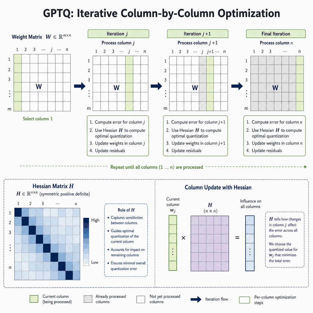
GPTQ (GPT Quantization) treats quantization as an optimization problem. Instead of applying a static formula, it greedily minimizes the reconstruction error of the layer's output.

Mechanism: GPTQ approximates the Hessian matrix (second-order derivatives) of the loss function with respect to the weights. It processes weights column-by-column. For each column, it calculates the optimal integer values that minimize the error relative to the previous layer's activations, assuming the other columns are already quantized.

This is computationally expensive. GPTQ requires a calibration dataset (a small subset of training data) to compute the Hessian approximation. The process is iterative and serial, making calibration times long (hours for large models).

Key Artifact: The auto-gptq library implements this. It produces models compatible with transformers via AutoGPTQForCausalLM.

Trade-off: GPTQ typically achieves the highest accuracy among post-training quantization (PTQ) methods, often matching FP16 performance closely. However, its deployment involves significant friction: while it produces high-fidelity INT4 weights, these do not always map directly to universally available hardware-optimized INT4 kernels. Unlike AWQ, which leverages native hardware support, GPTQ often requires specific custom CUDA kernels (like those in auto-gptq) that are not present on all hardware configurations, limiting its ease of deployment compared to more general-purpose solutions.

AWQ: Activation-Aware Weight Quantization

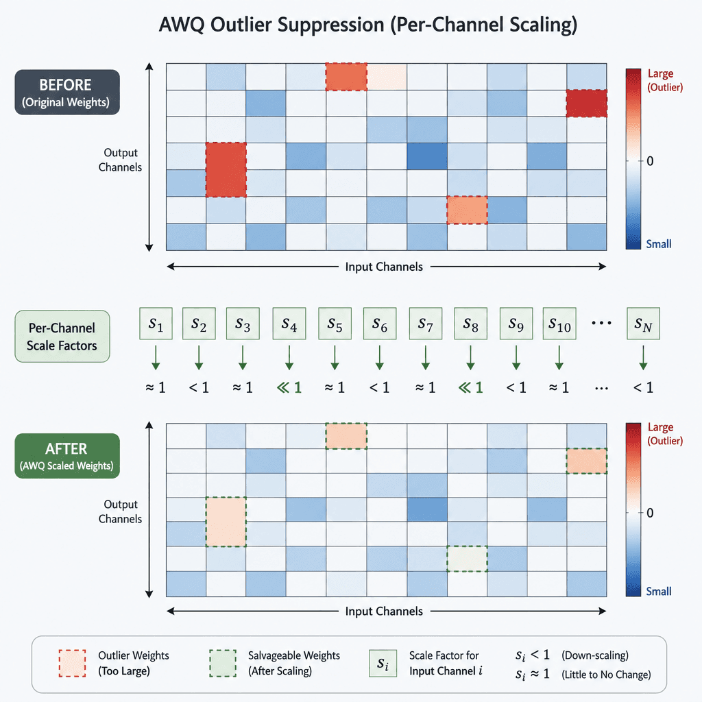
AWQ (Activation-Aware Weight Quantization) addresses the outlier problem by identifying the relationship between specific weights and activation outliers.

Mechanism: AWQ operates on the observation that large activations (outliers) are primarily caused by specific large weights. AWQ identifies these "salient" weights—those with the highest absolute magnitude. Instead of forcing them into a small quantization bin, AWQ scales them up (via a per-channel scaling factor, with the corresponding activations scaled down) to preserve the overall dynamic range.

Specifically, AWQ uses a layer-wise optimization to find a scale factor $S$ for each layer such that the quantization error is minimized. It essentially "compresses" the dynamic range by treating outliers as special cases rather than noise.

Key Artifact: The llm-awq library. It provides pre-calibrated models and tools for custom calibration.

Trade-off: AWQ calibration is faster than GPTQ because it does not require Hessian computation. More importantly, AWQ models are designed to work with hardware-accelerated INT4 kernels (e.g., on NVIDIA Ampere/Hopper architectures). This often results in faster inference than GPTQ on supported hardware, with accuracy losses slightly higher than GPTQ but lower than naive quantization.

Bitsandbytes: NormalFloat4 and Linear Quantization

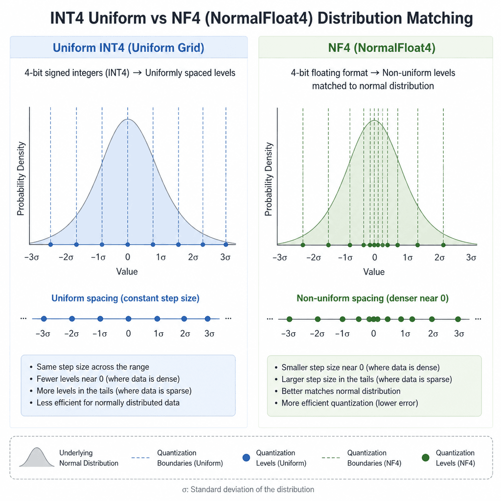
Bitsandbytes (BnB) takes a different approach. It does not perform complex layer-wise optimization or outlier suppression. Instead, it focuses on the quantization format itself.

Mechanism: Bitsandbytes popularized NF4 (NormalFloat4), a quantization scheme designed specifically for the Gaussian distribution of LLM weights. Unlike uniform INT4, NF4 uses 16 unique quantization levels that are optimally spaced according to the cumulative distribution function (CDF) of a normal distribution. This means more quantization levels are placed where the probability density is high (near zero) and fewer where it is low (tails).

For inference, BnB often uses INT8 or NF4 linear layers. The key advantage is lazy loading: BnB can quantize models on-the-fly during the load process, eliminating the need for a separate, time-consuming calibration phase before deployment. This makes it the fastest method to get a quantized model running, since it does not require a dedicated calibration dataset or iterative optimization loop beforehand.

Key Artifact: The bitsandbytes library. It integrates with transformers via load_in_4bit or load_in_8bit.

Trade-off: The primary benefit is ease of use and speed of deployment. You can load a model and start experimenting immediately. However, NF4 inference can be slower than INT4 on some hardware due to the complexity of dequantizing non-uniform grids. Accuracy is generally good but may lag behind GPTQ/AWQ on very tight quantization levels (e.g., below 4-bit) because it lacks the fine-grained outlier handling of the other two methods.

Practical Comparison: Choosing the Right Tool

The quantization comparison for ML engineers should be based on three factors: hardware support, calibration resources, and accuracy requirements.

Feature	GPTQ	AWQ	Bitsandbytes (NF4/INT8)
Calibration	Slow (Hessian-based)	Medium (Layer-wise opt)	Instant (No calibration)
Accuracy	Highest (PTQ)	High	Good (Depends on bits)
Inference Speed	Variable (Kernel dependent)	Fast (Hardware INT4)	Moderate (Dequant overhead)
Hardware Support	Custom CUDA required	NVIDIA Ampere/Hopper	Any GPU (CPU fallback)
Use Case	Max accuracy, offline cal	Production, NVIDIA GPUs	Quick prototyping, CPU/Edge

Scenario 1: Production on NVIDIA A100/H100 Choose AWQ. The hardware supports native INT4 matrix multiplication, which is significantly faster than dequantizing NF4. The calibration time is acceptable, and the accuracy is sufficient for most downstream tasks.

Scenario 2: Maximum Accuracy for Research Choose GPTQ. If you have a small calibration dataset and can afford the calibration time, GPTQ will yield the lowest perplexity. It is the gold standard for post-training quantization when accuracy is paramount.

Scenario 3: Rapid Prototyping or CPU Inference Choose Bitsandbytes. You can load any model with load_in_4bit and start experimenting immediately. While slower than hardware-optimized INT4, it is far faster than running FP16 on CPU. For CPU, BnB's INT8 is often the only viable quantization option due to lack of specialized INT4 kernels.

Conclusion

The quantization comparison reveals that no single method dominates all metrics. GPTQ optimizes for accuracy through second-order calculus. AWQ optimizes for hardware efficiency through outlier suppression. Bitsandbytes optimizes for accessibility through distribution-matched formats. Understanding the calibration and mechanism behind each allows you to select the tool that aligns with your hardware constraints and latency requirements.

For most production deployments on modern NVIDIA GPUs, AWQ offers the best balance of speed and accuracy. For research or maximum fidelity, GPTQ remains the benchmark. For quick iteration or CPU-bound environments, Bitsandbytes provides the lowest barrier to entry.