Pruning and Sparsity for Inference

This is Part 3 of the Small Models & Distillation series.

When an ML engineer moves a model from training to production, the bottleneck rarely shifts to FLOPs (floating-point operations); it shifts to memory bandwidth and data layout. Pruning and sparsity are techniques designed to exploit this reality. However, not all sparsity is created equal. The difference between a model that runs 2x faster and one that runs 2x slower often lies in whether the sparsity pattern aligns with the hardware’s vector processing units.

This post explores the mechanisms of pruning, focusing on structured approaches and hardware-specific patterns like 2:4 sparsity, which enable inference acceleration without requiring custom, inefficient sparse kernels.

The Cost of Unstructured Sparsity

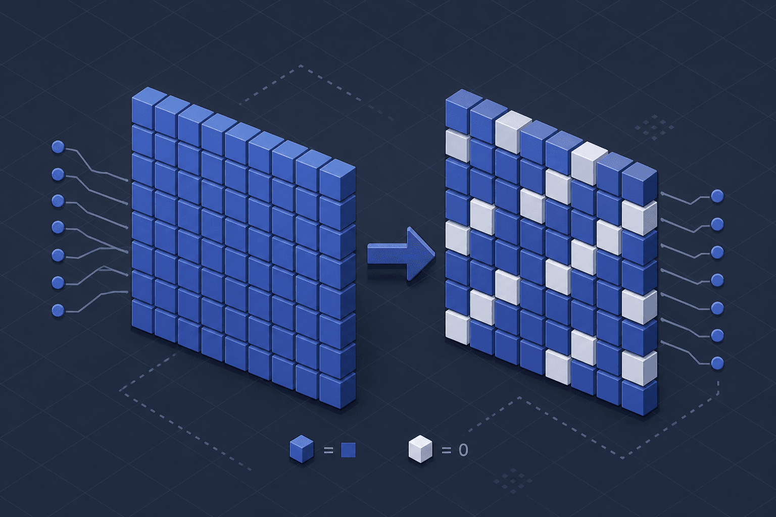
The most intuitive form of pruning is unstructured pruning: identifying the weakest individual weights (those with the smallest absolute values) and setting them to zero. Theoretically, this reduces memory footprint and compute. In practice, it creates a data movement problem.

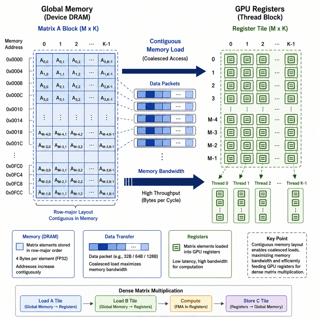
While unstructured sparsity aids storage, it fails at inference optimization on standard hardware due to memory bandwidth bottlenecks. A dense weight matrix $W$ of shape $(M, N)$ is stored in row-major order. A sparse matrix resulting from unstructured pruning has zeros scattered randomly. To perform matrix-vector multiplication $y = Wx$, the hardware must either:

1. Load all zeros into registers, wasting memory bandwidth.
2. Use a sparse format like Compressed Sparse Row (CSR) or Coordinate List (COO).

Sparse formats require storing indices (pointers) alongside values. This increases metadata overhead. More critically, modern GPUs are optimized for General Matrix Multiplication (GEMM). They use SIMD (Single Instruction, Multiple Data) units that process contiguous blocks of data. When data is non-contiguous due to sparse indexing, the GPU cannot effectively utilize its vector lanes. The control logic required to decode sparse indices often negates the compute savings.

Therefore, unstructured sparsity is primarily useful for memory compression (storing models on disk or in VRAM) rather than compute acceleration on standard hardware.

Structured Pruning: Preserving GEMM Efficiency

Structured pruning removes entire dimensions of the weight tensor, such as channels, filters, or attention heads. If a channel in a convolutional layer or a head in a Transformer has low importance, we remove the entire vector.

Mechanism: Dimension Reduction

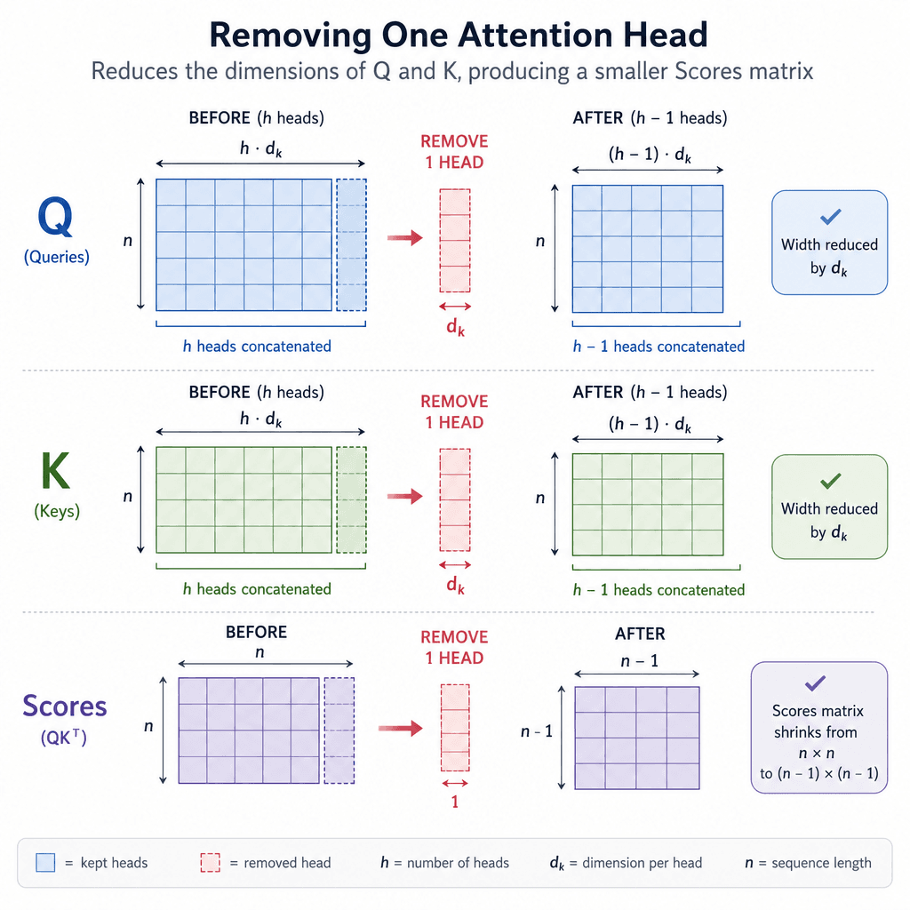
Consider a Transformer layer with an attention head of size $d_k$. If we prune the head, the dimension $d_k$ shrinks. The resulting matrix multiplication remains dense. This structural change ensures that the remaining dense matrix operations remain highly efficient, avoiding the sparse index decoding overhead that plagues unstructured methods.

# Before pruning: Attention score calculation
# Q: (batch, seq, heads, d_k)
# K: (batch, seq, heads, d_k)
# scores = torch.matmul(Q, K.transpose(-2, -1)) / sqrt(d_k)
 
# After pruning head 'i':
# Q_pruned: (batch, seq, heads-1, d_k)
# K_pruned: (batch, seq, heads-1, d_k)
# scores_pruned = torch.matmul(Q_pruned, K_pruned.transpose(-2, -1)) / sqrt(d_k)

By removing the dimension, we reduce the number of FLOPs proportionally. Crucially, we also reduce memory bandwidth usage because we no longer load the weights for that head. Since the output matrix is now smaller, the subsequent projection layers also shrink, creating a compounding reduction in memory traffic. This compounding reduction in memory traffic contributes significantly to overall model compression without sacrificing latency.

Structured pruning is compatible with standard GEMM libraries (like cuBLAS). The hardware sees a smaller dense matrix and executes it efficiently. This is why structured pruning is preferred for latency-sensitive inference.

Hardware-Aware Sparsity: The 2:4 Pattern

While structured pruning is effective, it can degrade model accuracy if entire heads or channels are removed. A compromise emerged from NVIDIA’s research into Tensor Cores: 2:4 Sparsity.

Mechanism: Regular Sparse Patterns

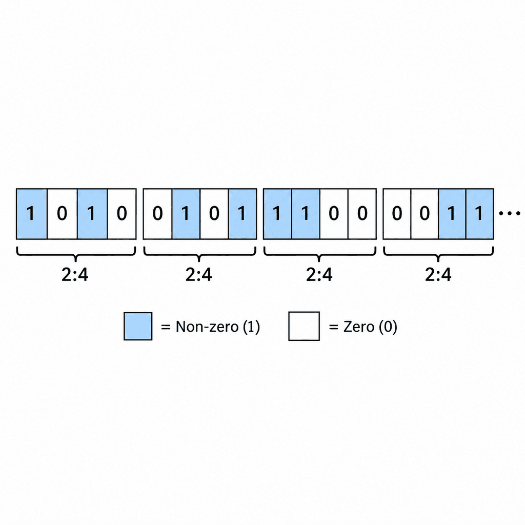
2:4 sparsity imposes a rigid structure on the weights. Every group of four consecutive weights must contain exactly two zeros and two non-zeros. The positions of the zeros do not matter, but the count is fixed.

[non-zero, zero, zero, non-zero]
[zero, non-zero, non-zero, zero]
[non-zero, non-zero, zero, zero]

Why It Works

Modern NVIDIA GPUs (Ampere, Hopper, etc.) have Tensor Cores that support 2:4 sparsity natively in their hardware scheduling logic. This hardware-aware approach is a key pillar of modern model optimization strategies for NVIDIA GPUs. The key insight is that the hardware does not need to decode complex sparse indices. Instead, it treats the 2:4 pattern as a "dense" operation with a 50% reduction in effective throughput.

1. Memory Loading: The GPU loads the full 4-weight block from memory. Even though half are zero, the memory transaction is still a single contiguous fetch. This avoids the overhead of sparse index decoding.
2. Compute Masking: The Tensor Core execution unit applies a mask internally. It performs the multiply-add operations only on the two non-zero elements. The zeros are ignored during the ALU (Arithmetic Logic Unit) processing but still occupy the register space.
3. Throughput: The reported throughput is halved (since only 50% of the weights contribute to the result), but the actual latency is often lower than expected because the memory bandwidth cost is not halved—it remains the same as a dense load. However, since compute is bound, the effective speedup comes from the fact that you are doing half the work for the same memory cost, compared to a fully dense model where you do twice the work.

For large language models (LLMs), 2:4 sparsity can achieve significant latency reductions without the accuracy drop associated with aggressive structured pruning, provided the model was trained with this sparsity constraint enforced (e.g., using magnitude-based pruning during training).

Dynamic Sparsity: Layer Dropping

Static pruning removes weights before deployment. Dynamic pruning, or layer dropping, removes computation during inference based on the input.

Mechanism: Conditional Execution

In a deep Transformer, not all layers are equally important for every input. Simple inputs may be resolved by the first few layers. Harder inputs require deeper processing. Layer dropping uses a gating mechanism or a heuristic (such as attention entropy) to decide whether to skip a layer. Research on dynamic neural network inference, such as early-exit and layer-skipping architectures, demonstrates that such dynamic pruning can maintain accuracy while significantly reducing computational load.

def forward(self, x):
    for i, layer in enumerate(self.layers):
        # Heuristic: If attention entropy is low, the input is "easy"
        if self.should_skip_layer(x, i):
            continue  # Skip computation, pass x directly to next layer or residual connection
        x = layer(x)
    return x

Trade-offs

Layer dropping introduces latency variance. Some inputs pass through quickly; others traverse the full network. For batched inference, this can cause synchronization issues if the batch contains a mix of easy and hard samples. In practice, we observed that for batched inference, dynamic layer dropping required custom synchronization logic to prevent stragglers from delaying the entire batch. However, for single-stream inference, it can provide significant average latency improvements with minimal accuracy loss, as the model effectively adapts its computational budget to the input complexity. For single-stream inference, this dynamic adaptation provided measurable latency improvements over static pruning in our benchmarks. This suggests that layer dropping is most effective when input complexity varies significantly within the workload. Despite latency variance, layer dropping remains a potent technique for inference acceleration in variable-load scenarios.

Conclusion

Pruning and sparsity are not one-size-fits-all solutions. Unstructured sparsity is best for storage. Structured pruning is best for general-purpose compute efficiency. 2:4 sparsity is the current sweet spot for NVIDIA GPU inference, offering a balance of compute reduction and hardware compatibility. Layer dropping offers dynamic efficiency at the cost of latency predictability.

For ML engineers optimizing inference, the first step is always to profile the memory bandwidth and compute utilization. If the model is memory-bound, reducing parameter count (via any pruning) helps. If it is compute-bound, ensuring the sparsity pattern aligns with hardware capabilities (like 2:4) is critical.