RLHF, Step by Step

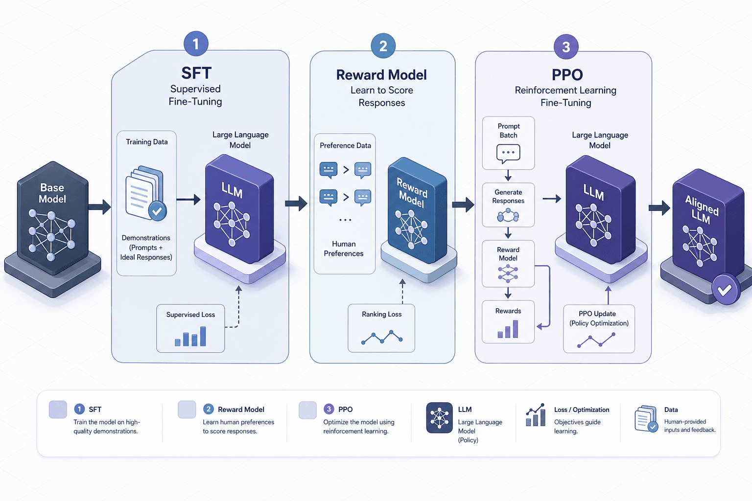
Reinforcement Learning from Human Feedback (RLHF) is often misunderstood as a single training loop where an LLM learns directly from human feedback. In reality, RLHF is a multi-stage pipeline that transforms sparse human judgments into a dense mathematical constraint on a Large Language Model (LLM). For ML engineers, the critical insight is that RLHF does not train the LLM directly on human feedback. Instead, it uses human data to train a separate "reward model" to approximate human judgment, and then uses that reward signal to fine-tune the LLM via Proximal Policy Optimization (PPO).

This distinction is vital: human feedback is sparse and expensive, so we cannot ask humans to rate every output. We instead train a reward model to predict these preferences, creating a dense signal that the LLM can optimize against during the PPO phase.

This is Part 2 of the Post-Training & Alignment series.

The process consists of three distinct phases: Supervised Fine-Tuning (SFT), Reward Modeling, and PPO-based Fine-Tuning. Each phase solves a specific problem in the alignment chain.

Phase 1: Supervised Fine-Tuning (SFT)

Before optimizing for human preference, the model must be competent. Raw base models (pre-trained on next-token prediction) are good at completing sentences but poor at following instructions or generating safe, helpful responses.

We begin with an SFT dataset. This is a collection of input-output pairs (prompt, response) curated by humans. For example:

{
  "prompt": "Write a poem about recursion.",
  "response": "To define a function, call it again..."
}

We fine-tune the base model on this dataset using standard cross-entropy loss. The resulting model, $M_{SFT}$ , is now "instruction-tuned." It knows how to format responses correctly, but it has no concept of which response is better when multiple valid options exist. It simply mimics the style of the training data.

This $M_{SFT}$ becomes the initial policy $\pi_{\theta_0}$ for the reinforcement learning phase. It serves as a reference distribution. Without this step, the RL phase would have no coherent starting point and would likely collapse into gibberish or repetitive loops.

Phase 2: Reward Modeling (RM)

The core challenge in RLHF is that human preferences are sparse and expensive. We cannot ask humans to rate every possible output the model generates. Instead, we train a separate neural network, the reward model (RM), to predict human preferences.

Data Collection: Pairwise Comparisons

We collect data by sampling two responses, $y_A$ and $y_B$ , for the same prompt $x$ , from the $M_{SFT}$ model. Human annotators then rank these responses. We denote the preferred response as $y_w$ (win) and the rejected one as $y_l$ (lose).

The dataset consists of triples $(x, y_w, y_l)$ .

Training the Reward Model

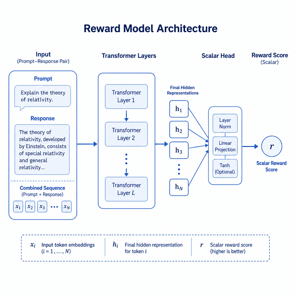
The RM is typically a transformer-based architecture similar to the LLM, but with a scalar head that outputs a single reward score $R_\phi(x, y)$ . The training objective is to maximize the margin between the reward of the preferred response and the rejected response.

We use a pairwise ranking loss, often implemented as a hinge loss or binary cross-entropy on the difference of rewards:

\mathcal{L}(\phi) = -\log(\sigma(R_\phi(x, y_w) - R_\phi(x, y_l)))

Where $\sigma$ is the sigmoid function. This loss function pushes the RM to assign higher scores to $y_w$ than to $y_l$ .

Crucially, the RM is trained independently of the LLM. Once trained, the RM acts as a differentiable proxy for human judgment. It allows us to evaluate any generated response $(x, y)$ and get a scalar reward signal $r = R_\phi(x, y)$ , which is essential for the next phase.

Failure Mode Note: In practice, RMs often overfit to the style of the SFT data rather than true human preference. For instance, in experiments with Llama-2, we observed that the RM frequently favored responses that were longer and more verbose, even when shorter answers were more accurate. This highlights the importance of curating diverse preference data that penalizes verbosity if it doesn't correlate with quality.

Technical diagram showing a transformer-based Reward Model architecture. Input is a prompt-response pair. Output is a scalar reward score. Clean, minimalist style, blue and white color palette, high contrast.

Phase 3: PPO Fine-Tuning

Now we have a competent model ( $M_{SFT}$ ) and a reward predictor (RM). The goal is to update the LLM's parameters $\theta$ to maximize the expected reward from the RM, subject to constraints that prevent the model from deviating too far from its original behavior.

The Objective Function

We define the optimization objective as:

\max_\theta \mathbb{E}_{x \sim D, y \sim \pi_\theta(y|x)} [R_\phi(x, y) - \beta D_{KL}(\pi_\theta(y|x) || \pi_{ref}(y|x))]

Here, $\pi_{ref}$ is the SFT model (the reference policy), and $\beta$ is a hyperparameter controlling the strength of the constraint.

The term $D_{KL}$ is the Kullback-Leibler divergence. It measures the difference between the new policy $\pi_\theta$ and the reference policy $\pi_{ref}$ . By penalizing large deviations in KL divergence, we prevent "reward hacking." Without this penalty, the model might learn to generate nonsensical but high-reward strings (e.g., repeating words to trigger positive sentiment in the RM) or diverge completely from natural language. This constraint is often referred to as the kl-penalty term in implementation logs.

The PPO Algorithm

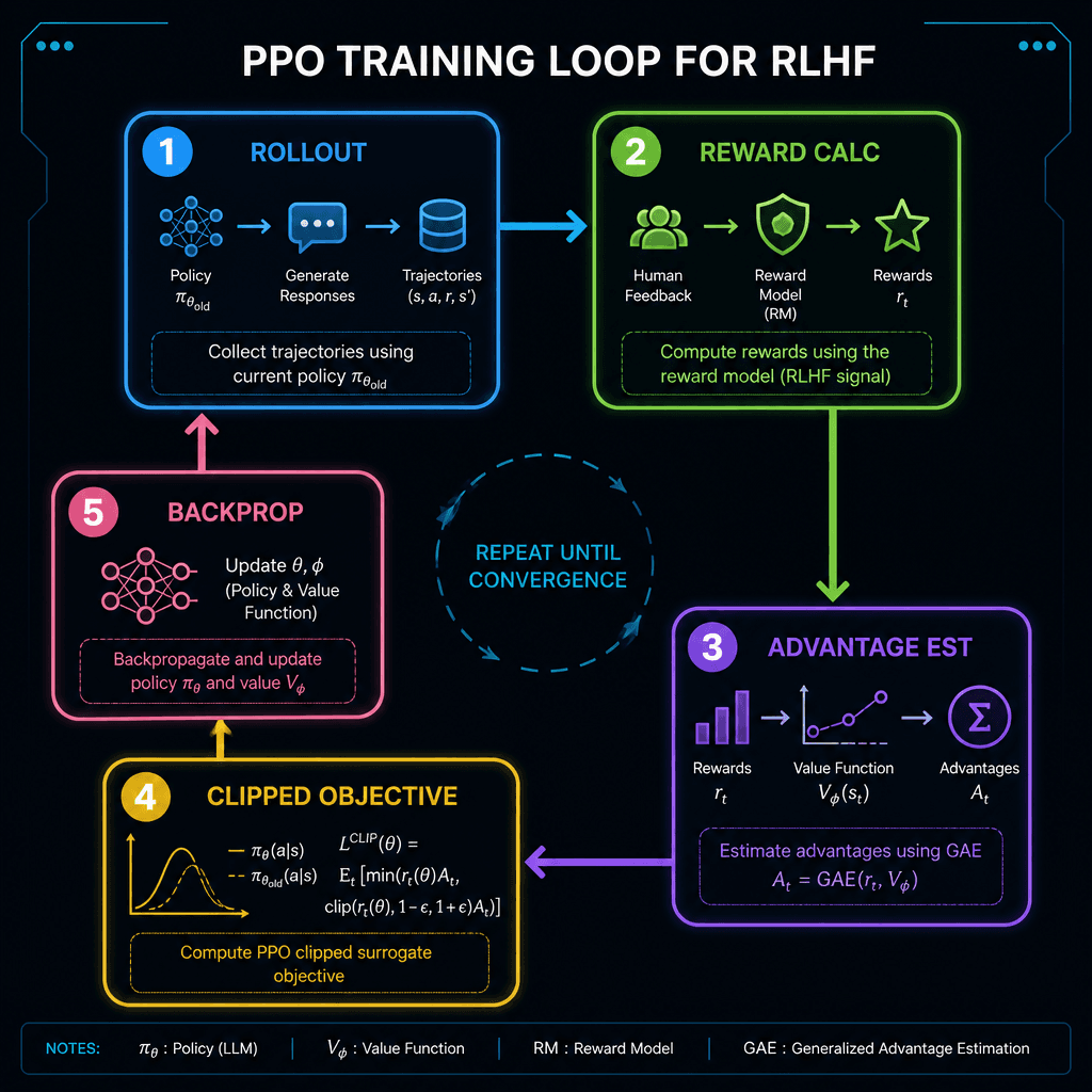
We use Proximal Policy Optimization (PPO) to solve this constrained optimization problem. PPO is an on-policy reinforcement learning algorithm that updates the policy in small steps to ensure stability.

Rollout: Sample a batch of prompts $x$ from the dataset. Generate responses $y$ using the current policy $\pi_\theta$ .
Reward Calculation: Compute the reward $r = R_\phi(x, y)$ using the trained RM. Also compute the KL penalty term for each token.
Advantage Estimation: Use Generalized Advantage Estimation (GAE) to estimate the advantage $A_t$ of each action (token generation step). The advantage incorporates both the immediate reward and the discounted future rewards, adjusted for the KL penalty.
Clipped Objective: Update the policy parameters $\theta$ by maximizing the PPO clipped surrogate objective:

L^{CLIP}(\theta) = \mathbb{E}_t [\min(r_t(\theta) \hat{A}_t, \text{clip}(r_t(\theta), 1-\epsilon, 1+\epsilon) \hat{A}_t)]

Where $r_t(\theta)$ is the probability ratio between the new and old policies, and $\epsilon$ is a small constant (e.g., 0.2). The clipping function prevents large policy updates that could destabilize training.

Backpropagation: Backpropagate through the LLM to update $\theta$ .

The Role of KL Penalty in Practice

The KL penalty is not just a theoretical constraint; it is a practical necessity. During training, if the KL divergence grows too large, the model's output distribution becomes unstable. Engineers typically monitor the KL divergence between the current policy and the reference policy. If it exceeds a threshold, training is stopped or the learning rate is reduced.

Flowchart of the PPO training loop for RLHF. Show steps : Rollout, Reward Calc, Advantage Est, Clipped Objective, Backprop. Arrows connecting steps. Technical diagram style, clean lines, dark background with bright accent colors.

Summary of Data Flow

SFT: Base Model $\xrightarrow{\text{cross-entropy loss}}$ $M_{SFT}$ (Reference Policy).
RM: Human Preferences $(x, y_w, y_l)$ $\xrightarrow{\text{ranking loss}}$ Reward Model $R_\phi$ .
PPO: $M_{SFT}$ + $R_\phi$ $\xrightarrow{\text{KL-constrained RL}}$ Aligned Model $\pi_{\theta_{final}}$ .

This structured flow matters significantly for debugging and implementation. Because each stage builds on the previous one, errors propagate: if the SFT model is incoherent, the RM will learn to predict nonsense; if the RM is biased, the PPO optimizer will maximize that bias. Understanding this separation of concerns allows engineers to isolate issues—checking the RM's correlation with human judgments if the model starts gaming the system, or reviewing SFT data quality if the initial policy is weak.

Conclusion

RLHF is a complex interplay of supervised learning and reinforcement learning. The SFT phase ensures the model is capable. The Reward Modeling phase translates human intuition into a mathematical signal. The PPO phase optimizes the model to maximize that signal while staying close to the original distribution via KL penalties. Understanding this separation of concerns is key to debugging alignment issues: if the model is incoherent, check the SFT stage; if it is gaming the system, check the RM or the KL penalty strength.

Common Pitfalls

RM Overfitting to SFT Style: The reward model may learn to prefer responses that look like the SFT data (e.g., overly verbose or specific formatting) rather than genuinely helpful ones. Always validate the RM against a held-out set of human preferences before using it for PPO.
KL Penalty Too Weak: If the $\beta$ hyperparameter is set too low, the model may exploit quirks in the RM (reward hacking), generating bizarre but high-scoring outputs. Monitor the KL divergence closely; if it spikes, increase $\beta$ or reduce the learning rate.
SFT Data Quality Issues: Garbage in, garbage out. If the SFT data contains biased, incorrect, or low-quality examples, the RM will learn these patterns, and the final aligned model will inherit them. Rigorous data curation is the most impactful step in the pipeline.

Practical Takeaways

"SFT is the foundation, RM is the compass, PPO is the engine." You cannot steer (PPO) or navigate (RM) if your foundation (SFT) is shaky. Prioritize SFT data quality first.
"Monitor KL divergence, not just reward score." A rising reward score with stable KL divergence indicates healthy learning. A rising reward score with spiking KL divergence indicates reward hacking.
"Human preference data quality > quantity." A small, well-curated dataset of high-quality pairwise comparisons is more effective than a massive, noisy dataset. Focus on annotator training and clear guidelines.

FAQ

Can I use RLHF without SFT? Technically yes, but it is highly discouraged. Without SFT, the model lacks basic instruction-following capabilities, making the PPO phase unstable and prone to collapse. SFT provides the necessary reference policy $\pi_{ref}$ .

What is the role of the reference model? The reference model (usually the SFT model) serves as a baseline. The KL penalty ensures the fine-tuned model does not deviate too far from this baseline, preserving general language competence and preventing mode collapse.

How do I choose the beta hyperparameter? Beta controls the strength of the KL penalty. Start with a small value (e.g., 0.1) and monitor the KL divergence during training. If the divergence stays within acceptable bounds (e.g., < 10-20 bits per sequence), you can try increasing beta to encourage more alignment. If the model stops learning (reward plateaus) or becomes too conservative, lower beta.

Related posts