Statistical Significance in LLM Evals

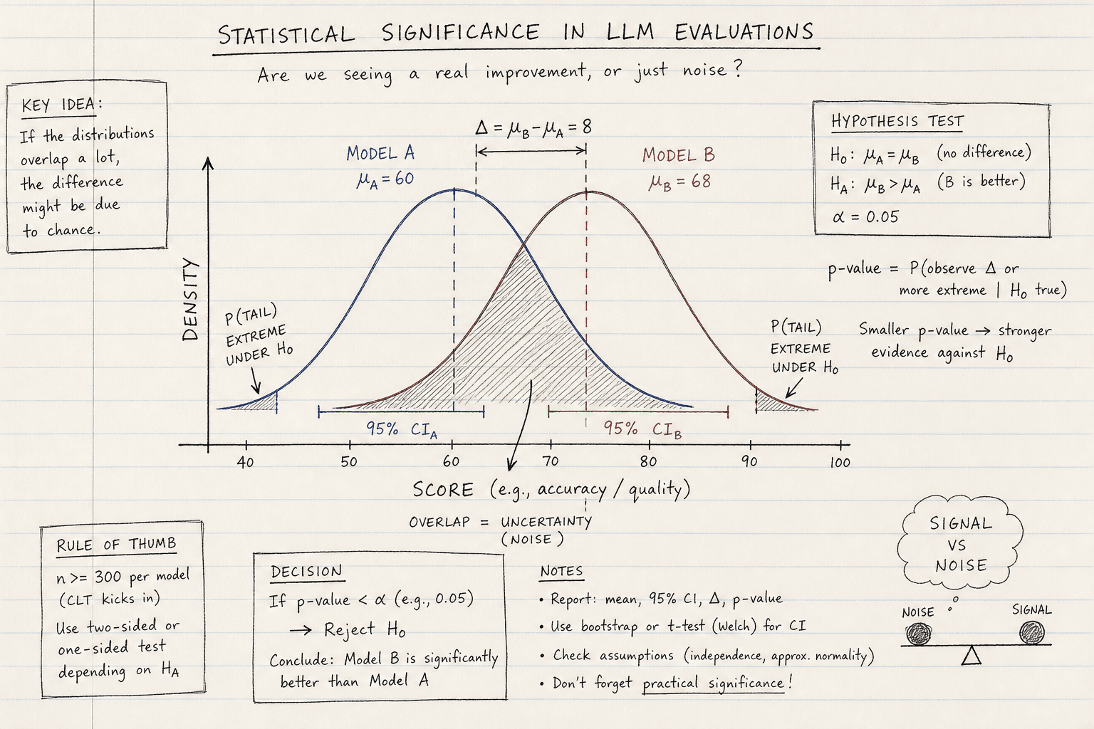
When you run an evaluation on a Large Language Model (LLM), you are not measuring a fixed property of the model. You are sampling from a probability distribution. The output of an LLM is influenced by temperature, top-p, and inherent randomness in the token generation process. Consequently, two runs of the same model on the same dataset will rarely yield identical scores. This variance is not a bug; it is a feature of the architecture.

Treating a single evaluation run as ground truth is a fundamental error. If Model A scores 85% accuracy and Model B scores 86% on a 50-prompt test set, you cannot conclude Model B is better. The difference might be within the noise floor of the evaluation harness. To distinguish signal from noise, you must apply statistical significance testing. This shifts evaluation from "what happened" to "what is likely true about the population."

The Variance Problem in Generative Metrics

In traditional software engineering, a unit test is deterministic. assert add(2, 2) == 4. In LLM evaluation, metrics like accuracy, BLEU, or human preference scores are random variables. While fixing the random seed makes generation deterministic for a specific run, variance still arises from non-deterministic system factors such as concurrency, hardware scheduling, or floating-point non-associativity in large context windows. This introduces variance in how different models interpret ambiguous instructions across different runs or environments.

The core challenge is that the metric of interest (e.g., binary accuracy) is a Bernoulli trial. If you evaluate $n$ prompts, the total score $S$ follows a Binomial distribution $B(n, p)$, where $p$ is the true accuracy. As $n$ grows, the distribution of the sample mean $\hat{p}$ approaches a Normal distribution due to the Central Limit Theorem (CLT). However, for small $n$ or extreme $p$ values (near 0 or 1), the normal approximation fails.

This means that a reported score of 90% is actually a point estimate with an associated error margin. Ignoring this margin leads to false positives: adopting a model that appears better but is statistically indistinguishable from the baseline.

Confidence Intervals: Quantifying Uncertainty

The first step in rigorous evaluation is calculating the confidence interval (CI). A 95% CI does not mean there is a 95% probability that the true mean lies within the interval. Rather, it means that if you repeated the experiment infinite times, 95% of the calculated intervals would contain the true population mean.

For a simple accuracy metric, you can estimate the standard error (SE) using:

$SE = \sqrt{\frac{\hat{p}(1-\hat{p})}{n}}$

The 95% CI is then approximately $\hat{p} \pm 1.96 \times SE$.

Consider two models evaluated on $n=100$ prompts.

• Model A: 85/100 correct ($\hat{p}=0.85$). $SE \approx 0.036$. CI: $[0.78, 0.92]$.
• Model B: 88/100 correct ($\hat{p}=0.88$). $SE \approx 0.033$. CI: $[0.82, 0.94]$.

The intervals overlap significantly. While Model B has a higher point estimate, the data is consistent with Model A being equal to or even slightly better than Model B. You cannot reject the null hypothesis that the models are equal based on this data alone.

To reduce the width of the CI, you must increase $n$. Because the margin of error scales with $1/\sqrt{n}$, doubling the sample size only reduces the error by ~30%. This is why small evals (n<50) are dangerously misleading. For robust LLM evals, aim for $n \geq 300$ for each model, depending on the expected effect size.

Hypothesis Testing: Paired Comparisons

When comparing two models, you should not treat them as independent samples. The same prompt tests both models. This pairing reduces variance because the difficulty of the prompt is a constant factor. Using an independent t-test or Z-test ignores this correlation, which inflates the variance of the difference estimator by failing to account for the positive correlation between paired observations. This increases the standard error, making it harder to detect real differences.

Instead, use McNemar’s Test for binary outcomes (correct/incorrect) or a Paired t-test for continuous scores (like LLM-as-a-judge scores).

McNemar’s Test Mechanism

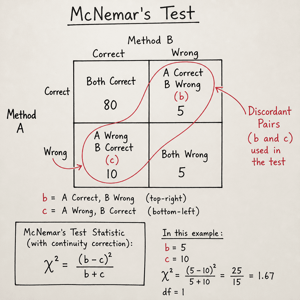
McNemar’s test focuses on the discordant pairs: cases where Model A is correct and Model B is wrong, and vice versa. Let $b$ be the count where A is correct and B is wrong, and $c$ be the count where A is wrong and B is correct. The test statistic is:

$\chi^2 = \frac{(b-c)^2}{b+c}$

This follows a Chi-squared distribution with 1 degree of freedom. If $b$ and $c$ are small, use the exact binomial version.

Example Scenario: You evaluate 100 prompts.

• Both correct: 80
• Both wrong: 5
• A correct, B wrong ($b$): 10
• A wrong, B correct ($c$): 5

Here, $b=10, c=5$. The test statistic is $(10-5)^2 / (10+5) = 25/15 = 1.67$. The critical value for $\alpha=0.05$ is 3.84. Since $1.67 < 3.84$, we fail to reject the null hypothesis. Despite Model A having more correct answers overall (90 vs 85), the difference is not statistically significant because the discordant pairs are too few to rule out chance.

Bootstrap Resampling for Complex Metrics

Not all metrics are binary. LLM-as-a-judge scores, latency, or token counts often have skewed distributions. The normal approximation may not hold. In these cases, bootstrap resampling is the most robust method.

Bootstrap works by empirically estimating the sampling distribution of your metric.

Algorithm:

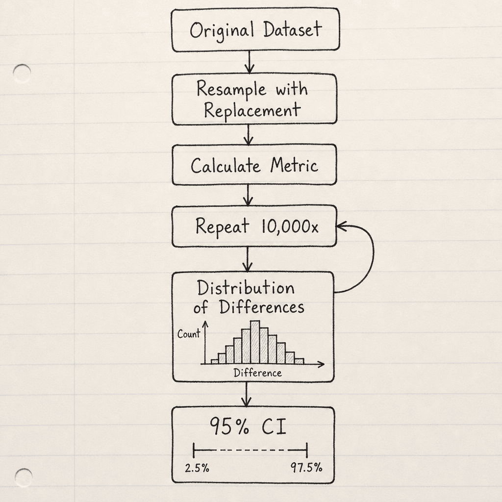
1. Start with your original dataset of $n$ results (e.g., scores for Model A and Model B).
2. Resample the dataset with replacement to create a new dataset of size $n$.
3. Calculate the metric of interest (e.g., mean difference in scores) for this bootstrap sample.
4. Repeat steps 2-3 thousands of times (e.g., 10,000 iterations).
5. The distribution of these 10,000 differences approximates the true sampling distribution.
6. The 2.5th and 97.5th percentiles of this distribution form the 95% CI for the difference.

If the 95% CI for the difference between Model A and Model B does not include zero, you have statistical significance.

Code Example (Python/Pandas):

import numpy as np
import pandas as pd
 
def bootstrap_ci(scores_a, scores_b, n_bootstrap=10000, alpha=0.05):
    diff_means = []
    for _ in range(n_bootstrap):
        # Resample with replacement
        sample_a = np.random.choice(scores_a, size=len(scores_a), replace=True)
        sample_b = np.random.choice(scores_b, size=len(scores_b), replace=True)
        # Calculate difference in means
        diff_means.append(np.mean(sample_a) - np.mean(sample_b))
    
    # Calculate CI
    lower = np.percentile(diff_means, 100 * alpha / 2)
    upper = np.percentile(diff_means, 100 * (1 - alpha / 2))
    return lower, upper
 
# Example usage
scores_a = [0.8, 0.9, 0.7, 0.85, ...] # List of judge scores
scores_b = [0.82, 0.88, 0.75, 0.84, ...]
 
ci_lower, ci_upper = bootstrap_ci(scores_a, scores_b)
print(f"95% CI for difference: [{ci_lower}, {ci_upper}]")

Sample Size Planning

Determining the required sample size beforehand prevents underpowered studies. The key parameter is the Effect Size. How large a difference do you care about detecting? If Model A is 80% and Model B is 80.1%, the difference is statistically detectable with a huge sample, but practically irrelevant.

Use power analysis to determine $n$. For a two-proportion z-test, the formula involves:

• $\alpha$ (significance level, usually 0.05)
• $\beta$ (power, usually 0.80, so $1-\beta = 0.80$)
• $p_1, p_2$ (expected proportions)

$n = \frac{(Z_{\alpha/2} + Z_{\beta})^2 \cdot (p_1(1-p_1) + p_2(1-p_2))}{(p_1 - p_2)^2}$

If you expect a small effect size (e.g., 2% improvement), $n$ will be large (hundreds or thousands). If you expect a large effect size (e.g., 10%), $n$ can be smaller. Always plan your evals with the minimum detectable effect in mind.

Conclusion

Statistical significance is not optional in LLM evaluation. It is the mechanism that separates signal from the inherent stochasticity of generative models. By using confidence intervals to quantify uncertainty, paired tests to leverage correlated data, and bootstrap methods for complex metrics, you ensure that your model selection decisions are defensible. Never report a point estimate without its error margin. If the intervals overlap, the models are effectively tied. If they don’t, you have evidence of improvement.