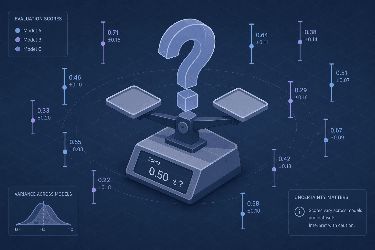
Why Your Eval Suite Is Lying to You

This is Part 1 of the "LLM Evaluation Engineering" series.

You run an evaluation. Model A scores 92% on your benchmark. Model B scores 88%. You ship Model A. Two weeks later, users complain about regression. You re-run the eval. Model A is now at 89%, Model B at 90%. Your suite didn’t lie; it just lacked the statistical resolution to distinguish signal from noise.

LLM evaluation is not a measurement of a static property like weight or latency. It is a measurement of a stochastic process. Every time you call an LLM, you are sampling from a probability distribution. When your sample size (N) is small, or when the output variance is high, the mean score you report is a poor estimator of true performance. This post explains the mechanism of that failure and how to build evals that resist false confidence.

The Variance Mechanism

Consider a simple classification task: identifying whether a customer support ticket is "urgent" or "routine." You have two models, TinyLLM-v1 and TinyLLM-v2. You test them on 10 representative tickets.

TinyLLM-v1 answers 9 correctly. TinyLLM-v2 answers 8 correctly.

You conclude the eval suite favors v1. But LLMs are non-deterministic. Even with temperature=0, some models exhibit minor variations due to system-level randomness or floating-point non-determinism across hardware. More critically, if you increase temperature to 0.7 for more creative reasoning, variance explodes.

Let’s say TinyLLM-v2 is actually more robust but happened to fail on the specific edge cases in your small test set. If you re-run the same 10 tickets, v2 might score 10/10 or 6/10. The standard deviation of its scores is high. Reporting only the mean (80%) hides the fact that its performance is unstable.

Mechanism: The observed score $S$ is a random variable. The true performance $\mu$ is unknown. The variance $\sigma^2$ determines how much $S$ fluctuates around $\mu$. High variance means you need many more samples to estimate $\mu$ accurately.

Sample Size and the Confidence Interval

The core error in most eval suites is treating a percentage as a precise number. In statistics, a percentage from a finite sample is an estimate with an error margin.

If you evaluate 50 prompts and get 45 correct (90%), what is the true accuracy? It is not exactly 90%. Using the Wilson Score Interval (preferred over the normal approximation for small N), we can calculate the 95% confidence interval.

For N=50, p=0.9:

• Lower bound: ~80.6%
• Upper bound: ~95.4%

Your reported score of 90% could be as low as 80.6% in reality. This is a massive range. If Model B scores 85% on the same 50 prompts, its interval might be [74%, 91%]. The intervals overlap significantly. You cannot claim Model A is better.

Worked Scenario:

1. You have 100 test cases.
2. Model X gets 95/100 correct.
3. Model Y gets 90/100 correct.
4. Calculate 95% CI for X: [89.2%, 98.3%].
5. Calculate 95% CI for Y: [83.1%, 95.1%].
6. The intervals overlap. The difference is not statistically significant at the alpha=0.05 significance level.

Most eval suites report only the point estimate. They omit the error bar. This creates the illusion of precision where none exists.

The Compound Noise of Automated Grading

Many modern evals use an LLM as a judge (e.g., "Does this response follow the instructions?"). This introduces a second layer of variance.

Let $M$ be the model under test. Let $J$ be the judge model.

The observed score is $Score(M, J)$. Both $M$ and $J$ are stochastic. The total variance is approximately:

$\sigma^2_{total} \approx \sigma^2_M + \sigma^2_J$

If your judge model is inconsistent (high $\sigma^2_J$), you need a larger N to compensate. A judge that flips labels on ambiguous inputs will inflate the apparent variance of your model, making it harder to detect real improvements.

Key Insight: You cannot separate the model’s performance from the judge’s noise without multiple evaluations per prompt or using a deterministic judge (like regex or exact match) where possible.

Building Reliable Evals

In machine learning, reliable evaluation is critical. To stop lying to yourself, apply these engineering practices:

1. Increase N Until Convergence

Don’t stop at 50 prompts. Run your eval until the confidence interval width stabilizes. For high-stakes applications, N should often exceed 500. Use a stopping criterion: stop when the margin of error is below your desired threshold (e.g., ±2%).

2. Report Confidence Intervals, Not Just Means

Every metric should be reported as mean ± CI. If your dashboard shows a line chart of accuracy over time, add shaded regions for confidence intervals. If the bands overlap, the change is likely noise.

3. Use Bootstrapping for Small Samples

If you have limited data, use bootstrapping. Resample your test set with replacement 1000 times, compute the mean for each resample, and take the 2.5th and 97.5th percentiles of those means as your CI. This works well for non-normal distributions.

import numpy as np
 
def bootstrap_ci(scores, n_bootstrap=1000, ci=0.95):
    means = []
    for _ in range(n_bootstrap):
        sample = np.random.choice(scores, size=len(scores), replace=True)
        means.append(np.mean(sample))
    lower = np.percentile(means, (1 - ci) / 2 * 100)
    upper = np.percentile(means, (1 + ci) / 2 * 100)
    return np.mean(scores), lower, upper

4. Stabilize Inputs

Reduce variance by fixing seeds where possible, but more importantly, by curating test sets that cover edge cases systematically. Random sampling from a large corpus is good, but targeted stratification ensures you’re measuring what matters. This is a common ai testing challenge, as ensuring coverage of rare but critical failure modes requires deliberate effort rather than random chance.

Common Pitfalls

1. Ignoring Judge Variance: Assuming the LLM-as-a-judge is deterministic. It is not. Always account for the judge's own error rate.
2. Overfitting to Small Test Sets: Chasing high scores on a tiny, curated set leads to models that perform well in evals but poorly in production.
3. Confusing Precision with Accuracy: High precision on a small set does not guarantee generalizable accuracy. Always look at the confidence interval width.

Practical Takeaways

1. Rule of Thumb: If CI overlaps, the models are tied. Do not make deployment decisions based on point estimates alone.
2. N is Not a Magic Number, but It Matters. While 50 might be enough for rough checks, 500+ is needed for statistical significance in most production scenarios.
3. Variance is Information. A high variance score tells you the model is unstable, which is often more important than the mean score itself.

FAQ

How small is too small for N? There is no single number, but for binary classification tasks, N < 30 typically yields confidence intervals wider than 10-15%, which is usually unacceptable for decision-making. Aim for at least 50-100 for rough comparisons, and 500+ for rigorous validation.

When should I use bootstrapping? Use bootstrapping when your data distribution is not normal (which is common in LLM scores) or when your sample size is too small for the Central Limit Theorem to guarantee that the mean follows a normal distribution.

Can I reduce variance without increasing N? You can reduce variance by stabilizing the judge (using more consistent prompts or deterministic fallbacks) and by stratifying your test set to ensure you are measuring consistent behaviors. However, you cannot eliminate sampling error entirely without increasing N.

Conclusion

Your eval suite is a statistical instrument. If you treat it like a ruler that gives exact measurements, you will be misled. LLM outputs are distributions, not points. By acknowledging variance, increasing sample sizes, and reporting confidence intervals, you transform your evals from vanity metrics into reliable decision-making tools. The goal is not to get a higher number; it is to know your number with certainty.

For further reading on the statistical methods mentioned:

• Wilson Score Interval: Refer to Wilson, E. B. (1927). "Probable inference, the law of succession, and statistical inference". Journal of the American Statistical Association.
• Bootstrapping: See Efron, B., & Tibshirani, R. (1993). An Introduction to the Bootstrap.