Roofline Analysis for LLM Serving

Large Language Model (LLM) serving presents a unique performance paradox. While training these models requires massive computational throughput, serving them is often constrained by data movement. Understanding this distinction is critical for ML engineers aiming to optimize GPU utilization. As Part 2 of the GPU Economics for AI Teams series, this guide introduces the roofline model as the mechanistic framework to visualize and quantify this constraint, moving beyond abstract metrics like "MFU" to reveal the physical bottleneck within the GPU architecture.

The Serving Bottleneck Mechanism

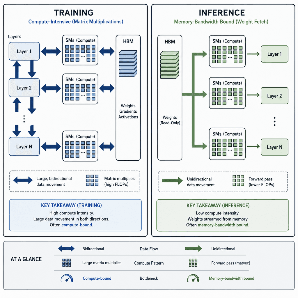
To apply the roofline model effectively, one must first understand the data flow difference between training and inference. During training, the GPU performs forward and backward passes, computing gradients for billions of parameters. This process is compute-intensive, meaning the GPU spends most of its time performing arithmetic operations (multiplications and additions). The workload sits near the "compute ceiling" of the roofline model chart.

Inference, however, operates differently. When a request arrives, the GPU must fetch the model weights from High Bandwidth Memory (HBM) into the Streaming Multiprocessors (SMs). For a 70B parameter model in FP16, this involves fetching 140 GB of data. If the sequence length is short, the number of arithmetic operations performed per byte fetched is low. The GPU core finishes the calculation almost instantly and then sits idle, waiting for the next chunk of weights to arrive from memory. This idle time is exacerbated by HBM read latency, which can be hundreds of cycles, and kernel launch overheads that further delay the start of computation.

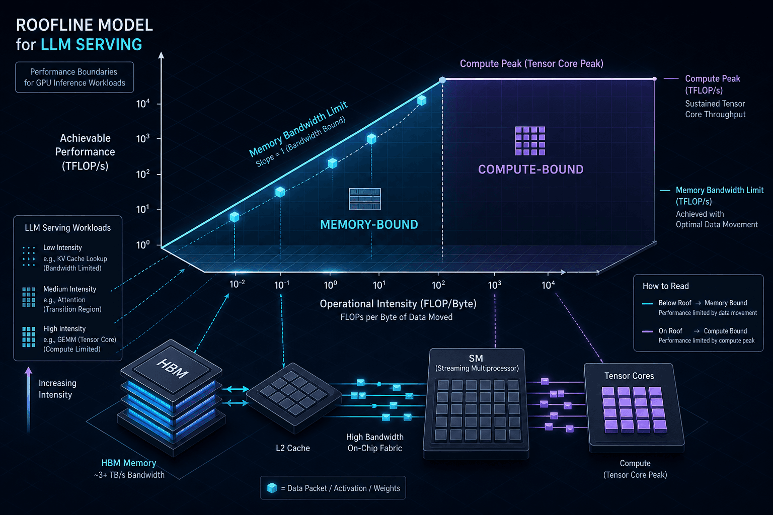
This creates a memory-bound regime. The performance is limited not by how fast the GPU can calculate, but by how fast it can move data. This is known as the "memory wall." In serving environments, especially with small batch sizes or short contexts, the system rarely reaches the compute ceiling. Instead, it operates along the diagonal slope of the roofline model chart, where performance scales linearly with memory bandwidth. This perspective is essential for effective performance analysis, as it highlights that reducing memory traffic is more impactful than increasing compute power in these scenarios.

Quantifying the Boundaries

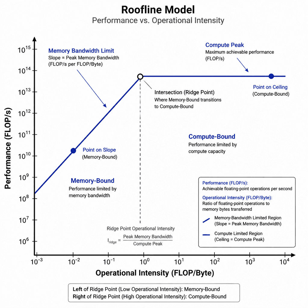
The roofline model plots two primary variables:

1. Performance (Y-axis): Measured in FLOPs per second (FLOP/s).
2. Operational Intensity (X-axis): Measured in FLOPs per byte (FLOP/Byte).

Operational intensity is the ratio of arithmetic work to data movement. For a single layer in a Transformer, we can derive this intensity. Consider a dense linear layer $Y = XW + b$. If the input sequence length is $S$, the hidden dimension is $H$, and the number of output units is $H$ (assuming square weight matrices for simplicity), the number of multiplications is roughly $2 \cdot S \cdot H^2$. The data movement involves reading the activation matrix ($S \times H$) and the weight matrix ($H \times H$).

$$\text{Intensity} = \frac{\text{FLOPs}}{\text{Bytes Moved}} \approx \frac{2 \cdot S \cdot H^2}{(S \cdot H + H^2) \cdot \text{precision\_bytes}}$$

As the sequence length $S$ increases, the numerator grows linearly, while the denominator also grows, but the weight matrix size ($H^2$) remains constant. This means that longer sequences increase operational intensity, pushing the workload toward the compute ceiling. Conversely, short sequences result in low intensity, keeping the workload on the memory-bound slope.

The "roof" itself is defined by two limits:

1. Memory Bandwidth Limit: $BW_{max}$ (e.g., 3 TB/s for NVIDIA H100). If the intensity is below the intersection point, performance is capped by bandwidth.
2. Compute Peak: $P_{max}$ (e.g., 989 TFLOPS for H100 FP16). If the intensity is above the intersection, performance is capped by arithmetic throughput.

This quantitative approach forms the basis of rigorous performance analysis in LLM serving, allowing engineers to predict how changes in batch size or sequence length will impact throughput.

From Theory to MFU

Model FLOPs Utilization (MFU) is a common metric in AI engineering, defined as the ratio of achieved performance to theoretical peak performance. However, MFU can be misleading if interpreted without context. A low MFU in a serving scenario does not necessarily indicate poor optimization; it may simply reflect the inherent inefficiency of the memory-bound regime.

The roofline model clarifies this by showing the theoretical maximum for a given operational intensity. If a model operates at an intensity where the theoretical roof is 50% of the peak compute power, achieving 90% of that theoretical maximum results in an overall MFU of 45%, which is actually excellent performance for that specific data movement profile.

Quantization techniques, such as moving from FP16 (2 bytes) to INT8 (1 byte), double the operational intensity by halving the data movement while keeping the arithmetic complexity similar. This shifts the operating point to the right on the X-axis, potentially crossing the intersection point into the compute-bound region. Note that INT8 operations are distinct from FLOPs (often called INT8-OPS or MACs) but represent equivalent arithmetic work volume. In this region, the GPU can utilize its full arithmetic throughput, leading to a significant jump in effective MFU.

Practical Diagnostic Workflow

To apply this roofline model analysis in a production serving environment, follow these steps:

1. Profile the Workload: Use tools like NVIDIA Nsight Systems or PyTorch Profiler to capture the timeline of a serving batch. Identify the dominant kernel operations (e.g., matmul, attention).
2. Measure Actual Intensity: Calculate the actual FLOPs executed and the bytes transferred during the kernel execution. This can be approximated by analyzing the tensor shapes and data types involved in the forward pass.
3. Plot on the Roofline: Map the measured performance (FLOP/s) and intensity (FLOP/Byte) onto the GPU's specific roofline model chart.
4. Identify the Gap: Determine if the point lies on the memory bandwidth slope or the compute ceiling.
   • On the slope: Optimize memory access patterns. Consider weight compression, better batching strategies to increase sequence length, or kernel fusion to reduce memory transactions.
   • On the ceiling: The model is compute-bound. Optimization should focus on increasing parallelism, using higher precision tensor cores, or reducing kernel launch overheads.

By treating the roofline model as a diagnostic map rather than a static benchmark, engineers can make targeted decisions about hardware selection and software optimization, ensuring that every dollar spent on GPU capacity translates into effective token generation.

Conclusion

Roofline model analysis provides the essential bridge between abstract performance metrics and physical hardware constraints in LLM serving. By distinguishing between memory-bound and compute-bound regimes, engineers can move beyond generic MFU numbers to implement targeted optimizations—whether that means improving data movement efficiency or maximizing arithmetic throughput. Understanding where your workload sits on the roofline model is the first step toward truly efficient GPU utilization.